COSI 21A Data Structures and Algorithms

Lecture 01 2022/01/19

Data Structure
- A data structure is a way to store and organize data in order to facilitate access and modifications
- No single data structure well for all purpose
- Each data structure has unique properties that make it well suited to a certain type of data
Algorithm
- An algorithm is any well-defined computational procedure that takes some value, or set ov values as input and produces some value, or set of values, as output
- Analysis of algorithm complexity:
  - Mathematical analysis
  - Independent of the machine the algorithm runs on, and the language used for programming
- Pseudocode: less formal than programming language, but more precise than English

Lecture 02 2022/01/20

Pseudocode

Description
- For human eyes only
- A mixture of natural language and high-level programming constructs
- Less detailed than a program
- Hides program design issues
- Preferred notation to describe algorithms

Syntax

Algorithm: should be titled to concisely describe what it does
Input and output: each algorithm must describe its input and output restrictions in English
Tabbing: no braces are used, tabs are used to indicate scope
Expressions
- Standard mathematical symbols for arithmetic and boolean expressions
- \(\leftarrow\) for assignment (equivalent to = operator)
- = used for equality (equivalent to == operator)

Control flow

-- if statement
if condition then
  statement
else
  statement
-- for loop
-- bothe the initial-value and final-value are inclusive
for variable <- initial-value to final-value do
  statement
-- while loop
while condition do
  statement

Array indexing: A[i]
Method call: variable.method(argument [, argument...])
Return value: return expression

Example

arrayMax(A, n)
  Input: array A of n integers. Array indexing starts from 0
  Output: maximum element of A

  res <- A[0]
  for i <- 1 to n - 1 do
    if A[i] > res then
      res <- A[i]
  return res

Cormen-lib project

Syntax

Expressions
- Standard mathematical symbols used for arithmetic and boolean expressions
- = used in assigned statements
- == used for equality

Control flow

# if statement
if condition:
  statement
else:
  statement
# for loop
# start is inclusive, stop is exclusive
for i in range(start, stop): 
  statement
# while loop
while condition:
  statement

Array syntax
- Instantiation: A = Array(n)
- Array indexing: A[i]

Example

def arrayMax(A):
  # Input: array A of n integers
  # Output: maximum element of A
  res = A[0]
  for i in range(1, A.length()):
    if A[i] > res:
      res = A[i]
  return res

Lecture 03 2022/01/24

Theoretical analysis
- General methodology
  - Consider all possible inputs
  - It can be performed studying high-level description of the algorithm
  - Evaluating the relative efficiency of algorithms is independent from hardware and software
- Assumptions
  - Memory is unlimited, all memory is equally expensive to access
  - Sequential execution
  - Support simple constant-time instructions
  - Support arithmetic operations, data movement and function calls
  - Memory access takes unit time
- Running time
  - The number of operations required to carry out a given task, it's open referred as time complexity
  - Running time is a function as input size n
- Primitive operations
  - Assign a value to a variable
  - Call a method
  - Perform an arithmetic operation
  - Compare two numbers
  - Index into an array
  - Return a value

Lecture 04 2021/01/26

Complexity of an algorithm depends on
- Size of input
- Other characteristics of the input data: is input sorted, is there cycles in the graph
Algorithm analysis
- Interested aspects:
  - Growth rate: how the running time grows with the input size
  - Asymptotic complexity: the running time for larger inputs
- Behaviors
  - Worst case: maximum time required for program execution
  - Average case: average time required for program execution
  - Best case: minimum time required for program execution
Asymptotic analysis
- Running time = \(f(n)\)
- Consider \(\lim\limits_{n\rightarrow \infty} \frac{f(n)}{g(n)}\)
- Exact running time/ exact complexity: a concrete form of \(f(n)\)
- Notation
  - \(O(n)\): \(\exists c > 0, n_0 > 1: \forall n \ge n_0, f(n) \le c * g(n)\)
  - \(\Omega(n)\): \(\exists c > 0, n_0 > 1: \forall n \ge n_0, f(n) \ge c * g(n)\)
  - \(\Theta(n)\): \(\exists c_1 > 0, c_2 > 0, n_0 > 1: \forall n \ge n_0, c_1 * g(n) \le f(n) \le c_2 * g(n)\)
- Common orders of magnitude
  - \(O(1)\): constant running time
  - \(O(logn)\): logarithmic running time
  - \(O(n)\): linear running time
  - \(O(nlogn)\): linearithmic running time
  - \(O(n^2)\):quadratic running time
  - \(O(n^3)\): cubic running time
  - \(O(n^k)\): polynomial running time
  - \(O(2^n)\): exponential running time

Lecture 05 2021/01/27

Asymptotic analysis
- Properties
  - Transitivity:
    - If \(f(n)\) is \(O(g(n))\), and \(g(n)\) is \(O(h(n))\), then \(f(n)\) is \(O(h(n))\)
    - If \(f(n)\) is \(\Omega(g(n))\), and \(g(n)\) is \(\Omega(h(n))\), then \(f(n)\) is \(\Omega(h(n))\)
    - If \(f(n)\) is \(\Theta(g(n))\), and \(g(n)\) is \(\Theta(h(n))\), then \(f(n)\) is \(\Theta(h(n))\)
  - Reflexivity:
    - \(f(n)\) is \(O(f(n))\)
    - \(f(n)\) is \(\Omega(f(n))\)
    - \(f(n)\) is \(\Theta(f(n))\)
  - Symmetry:
    - \(f(n)\) is \(\Theta(g(n)) \iff g(n)\) is \(\Theta(f(n))\)
  - Complementary:
    - \(f(n)\) is \(O(g(n)) \iff g(n)\) is \(\Omega(f(n))\)
- Useful Rules
  - If \(d(n)\) is \(O(f(n))\), then \(a*d(n)\) is \(O(f(n))\), for any constant a > 0
  - If \(d(n)\) is \(O(f(n))\), and \(e(n)\) is \(O(g(n))\), then \(d(n) + e(n)\) is \(O(f(n) + g(n))\)
  - If \(d(n)\) is \(O(f(n))\), and \(e(n)\) is \(O(g(n))\), then \(d(n) * e(n)\) is \(O(f(n) * g(n))\)
  - If \(d(n)\) is \(O(f(n))\) and \(f(n)\) is \(O(g(n))\), then \(d(n)\) is \(O(g(n))\)
  - If \(f(n)\) is a polynomial of degree d, then \(f(n)\) is \(O(n^d)\)

Lecture 06 2021/01/31

Stack
- A stack is a linear data structures
- It stores arbitrary elements according to the LIFO (last in first out) principle
- You can only access the top of the stack
- Stack can be implemented using array and linked-list
- Stack index starts from 1
- Operations
  - push(ele): insert an element
    1
    2
    3
    4
    5
    6
    7
    push (S, x):
    if S.top_index >= n then:
    Error: stack overflow
    else:
    S.top_index <- S.top_index + 1
    S[top_index] <- x
  - pop(): remove and return the last inserted element
    1
    2
    3
    4
    5
    6
    pop(S):
    if stack-Empty(S) then:
    Error: stack underflow
    else:
    S.top_index <- S.top_index - 1
    return S[S.top_index + 1]
  - top(): return the last inserted element without removing it
    1
    2
    3
    4
    top(S)
    if stack-Empty(S) then
    Error: stack empty
    return S[S.top_index]
  - size(): return the number of element stored
    1
    2
    size(S)
    return S.top_index
  - isEmpty(): indicate whether no elements are stored
    1
    2
    3
    4
    5
    stack-Empty(S)
    if S.top_index == 0 then
    return true
    else
    return false
- Performance
  - Space used: \(O(n)\)
  - Each operation runs in time: \(O(1)\)
Queues
- A queue is a linear data structure
- It stores arbitrary elements according to the FIFO (first in first out) principle
- You can insert an the end of the queue, and remove from the front of the queue
- Queue can be implemented using array and linked-lists
- Queue index starts from 1
- Queue implementation choice
  - Let index 1 be the front of the queue: not a good choice, each dequeue operation involves shifting the remaining elements, which is linear complexity
  - Use front_index(the current head element) and rear_index (rear_index - 1 is the current rear element): the pointers need to be wrapped around after reaching the end of the array, which results in a circular queue.
    For an array indexing from 1 to n, there can be at most n - 1 elements in the circular queue
- Operations
  - enqueue(ele): insert an element at the end of the queue
    1
    2
    3
    4
    5
    6
    enqueue(Q, x)
    if size(Q) = n then
    Error: queue overflow
    else
    Q[Q.read_index] = x
    Q.read_index < - Q.read_index % n + 1
  - dequeue(): remove and return the element at the front of the queue
    1
    2
    3
    4
    5
    6
    7
    dequeue(Q):
    if isEmpty(Q) then
    Error: queue underflow
    else
    x <- Q[Q.front_index]
    Q.front_index <- Q.front_index % n + 1
    return x
  - size(): return the number of element stored
    1
    2
    size(Q)
    return (n + Q.rear_index - Q.front_index) % n
  - isEmpty(): indicate whether no elements are stored
    1
    2
    3
    4
    5
    isEmpty(Q)
    if Q.front_index = Q.rear_index then
    return true
    else
    return false
  - rear()
    1
    2
    3
    4
    5
    6
    7
    8
    rear(Q)
    if isEmpty(Q) then
    Error: queue empty
    else
    if Q.rear_index = 1 then
    return Q[n]
    else
    return Q[Q.rear_index - 1]
  - front()
    1
    2
    3
    4
    5
    front(Q)
    if isEmpty(Q) then
    Error: queue empty
    else
    return Q[Q.front_index]
- Search in queue: \(O(n)\)

Lecture 07 2022/02/02

Examples
- Evaluating postfix
- Parentheses matching
- Reverse an array
- Separate an array
Array limitation
- Fixed size
- Physically stored in consecutive memory locations
- To insert or delete items, may need to shift data
Time complexity analysis
- Linear search: \(O(n)\)
- Binary search: the array needs to be sorted, \(O(logn)\)
- Bubble sort: \(O(n^2)\)

Lecture 08 2022/02/03

Introduction
- Array limitations
  - Fixed size
  - Physically stored in consecutive memory locations
  - To insert or delete items, may need to shift data
- A linked data structure consists of items that are linked to other items
- Advantages
  - Items do not have to be stored in consecutive memory locations
  - Linked lists can grow dynamically
Linked list
- A linked list L (or head) is a linear data structure consisting of nodes
- Linear or der of linked list is determined by a link to the next node
- A node consists of two fields
  - A data portion (called key or data), it should be generic
  - A link (or pointer) to the next node in the structure
- x.next points to the successor of node x
- x.next = NIL indicates that x is the last node in the linked list
- Singly linked list
  - It has one lik per node, which points to the next node in the list
  - The list has a link to the first node called L (or head), L = NIL indicates the list is empty
  - The list may or may not have a tail
- Link hopping: traversing the linked list by moving from one node to another via following the link next
- x.next = p: node p is the successor of node x
- p.next = x: node p is the predecessor of node x
- The length of a linked list is the number of nodes in the list
- Operations on linked list: isEmpty, insertNode, findNode, deleteNode, displayList
- Search in a linked list
  1
  2
  3
  4
  5
  6
  # Linear time complexity
  search(L, x)
  cur <- L
  while cur != NIL and cur.key != x do
  cur <- cur.next
  return cur

Lecture 09 2022/02/07

Linked list operations

Insert a node in the linked list

Insert a node in an empty linked list

# Constant time complexity
insertEmpty(L, x)
  p <- newNode()
  p.key = x
  p.next = NIL
  L <- p
  size <- size + 1

Insert a node at the beginning of a linked list

# Constant time complexity
insertFirst(L, x)
  p <- newNode()
  p.key = x
  p.next <- L
  L <- p
  size <- size + 1

Insert a node at the end of a linked list

# If we do not have a tail pointer
# Linear time complexity
insertLast(L, x)
  cur <= L
  while cur.next != NIL do
    cur <- cur.next
  p <- newNode()
  p.key = x
  p.next <- NIL
  cur.next <- p
  size <- size + 1

# If we have a tail pointer
# Constant time complexity
insertLast(L, tail, x)
  p <- newNode()
  p.key <- x
  p.next <- NIL
  tail.next <- p
  tail <- p
  size <- size + 1

Insert a node after a given node

# Constant time complexity
insertAfter(L, x, curNode)
  p <- newNode()
  p.key <- x
  p.next <- curNode.next
  curNode.next <- p
  size <- size + 1

Delete a node

Delete the first node

# Constant time complexity
deleteFirst(L)
  if L == NIL then
    Error: Linked list is empty
  L <- L.next
  size <- size - 1

Delete the last node

# Linear time complexity
deleteLast(L)
  if L = NIL then
    Error: Linked list is empty
  if L.next = NIL then
    L <- NIL
  cur <- L
  while cur.next != NIL and cur.next.next != NIL do
    cur <- cur.next
  cur.next = NIL
  size <- size - 1

Delete a node in the middle

# Constant time complexity
deleteMiddle(L, prev, curr)
  prev.next <- curr.next
  size <- size - 1

Reverse a linked list

# Iterative approach
reverseLink(L)
  if L == NIL or L.next == NIL then
    return L
  prv <- NIL
  cur <- L
  while cur != NIL do
    nxt <- cur.next
    cur.next <- prv
    prv<- cur
    cur <- nxt
  return prv

# Recursive approach
reverseLink(L)
  if L == NIL or L.next == NIL then
    return L
  # the function reverseLink(p) reverse the linked list starting from
  # node p, and return the new head of the reversed linked list
  p <- reverseLink(L.next)
  # L.next is the tail of the reversed list, so put L as the new tail
  L.next.next <- L
  L.next <- NIL
  return p

Lecture 10 2022/02/09

Static v.s. dynamic data structures
- Static data structure such arrays allow
  - Fast access to elements
  - Expensive to insert/remove elements
  - Have fixed, maximum size
- Dynamic data structure such ass linked list allow
  - Fast insertion/deletion of elements, no need to move other nodes, only need to reset some pointers
  - Slower access to elements, do not keep track of any index for the nodes
  - Can easily grow and shrink in size
Linked list implemented stack and queue
- Stack: space is \(O(n)\), each operation is \(O(1)\)
  - top(), push(), pop()
- Queue: space is \(O(n)\), each operation is \(O(1)\)
  - front(), rear(), enqueue(), dequeue()
Variations of linked list
- Doubly linked list
- Circular linked list
- Sorted linked list

Doubly linked list

Node
- x.data, d.next, x.prev
- x.prev = NIL, then x is the first element
- x.next = NIL, then x is the last element
- head points to the first element in the list
- head = NIL, then the list is empty

Insert at the front of a doubly linked list

# Constant time complexity
insertFirst(L, x)
  p <- newNode()
  p.key <- x
  p.prev <- NIL
  p.next <- L
  if L != NIL then 
    L.prev <- p
  L <- p
  size <- size + 1

Insert after a node

# Constant time complexity
insertAfter(L, x, cur)
  p <- newNode()
  p.key <- x
  p.prev <- cur
  p.next <- cur.next
  if cur.next != NIL then
    cur.next.prev <- p
  cur.next <- p
  size <- size + 1

Delete a node

# Constant time complexity
deleteNode(L, cur)
  if L = NIL or cur = NIL then
    Error: Cannot delete
  if cur.prev = NIL then
    L <- cur.next
  else
    cur.prev.next <- cur.next
  if cur.next != NIL then
    cur.next.prev <- cur.prev
  size <- size - 1

Lecture 11 2022/02/10

Introduction
- Recursion is a problem solving approach where the solution of a problem depends on solutions to smaller instances of the same problem
- Recursion uses the divide-and-conquer technique
Recursion problems
- A recursive description of a problem is one where
  - A problem can be broken into smaller parts
  - Each part is a smaller version of the original problem
  - There is a base case that can be solved immediately
- A recursive algorithm has at least two cases
  - Base case
  - Recursive case
- Tail recursion: when recursion involves single call that is at the end it is called tail recursion and is easy to make iterative
- Cost of recursion: call a function consumes more time and memory than adjusting a loop counter, thus high performance applications hardly ever use recursion

Lecture 12 2022/02/14

Analysis of recursive algorithm
- Recursive mathematical equations are called recurrence equations/ recurrence relations, or simply recurrence
- We use recurrence relation to analyze recursive algorithm
- Recurrence relation, \(T(n)\), is an equation which is defined in terms of itself \[T(n) = \begin{cases} c & \text{if n = 0 base case}\\ a*T(n) + b & \text{if n > 0 recursive case}\\ \end{cases}\]
  - a is the number of sub-problems
  - m is the size of the sub-problems
  - b is the time to divide into sub-problems and combine the solution
- Examples
  - Example 1
    1
    2
    3
    4
    5
    Foo(n)
    if n = 0 then
    return 2
    else
    return Foo(n - 1) + 5
    \[T(n) = \begin{cases} c & \text{if n = 1} \\ T(n - 1) + b & \text{if n > 1} \end{cases}\]
  - Example 2
    1
    2
    3
    4
    5
    Foo(n)
    if n = 1 then
    return 1
    else
    return Foo(n / 2) + Foo (n / 2) + 5
    \[T(n) = \begin{cases} c & \text{if n = 1}\\ 2 * T (n / 2) + b & \text{if n > 1} \end{cases}\]
  - Example 3
    1
    2
    3
    4
    5
    Foo(n)
    if n = 1 then
    return 1
    else
    return Foo(n - 1) + Foo(n / 2) + 5
    \[T(n) = \begin{cases} c & \text{if n = 1} \\ T(n - 1) + T(n/2) + b & \text{if n > 1} \end{cases}\]
Solving recurrence relations
- Example 1 \[T(n) = \begin{cases} 1 & \text{if n = 0}\\ b + T(n-1) & \text{else }\end{cases}\]
  - \(T(n) = n * b + 1\), so \(T(n)\) is linear complexity
- Example 2 \[T(n) = \begin{cases} 1 & \text{if n = 0 or n = 1}\\ T(n - 1) + T(n-1) & \text{else }\end{cases}\]
  - \(T(n)\) is exponential complexity
- Improved Fibonnacci
  1
  2
  3
  4
  5
  6
  7
  8
  # Linear time complexity
  improvedFibonnacci(n)
  a <- Array(n + 1)
  a[0] <- 1
  a[1] <- 1
  for i <- 2 to n do
  a[i] <- a[i - 1] + a[i - 2]
  return a[n]

Lecture 13 2022/02/16

Solving recurrence relation

Example 1 \[T(n) = \begin{cases} c & \text{if n = 1} \\ 2 * T(n/2) + b & \text{if n > 1}\end{cases}\]
- \(T(n) = c + (n - 1) * b\), so \(T(n)\) is linear complexity
Example 2 \[T(n) = \begin{cases} c & \text{if n = 1} \\ T(n - 1) + n + b & \text{if n > 1}\end{cases}\]
- \(T(n) = c + n * (n + 1) / 2 - 1 + n * (n - 1)\), so \(T(n)\) is quadratic complexity

Example 3: Binary search recursively

# Logarithmic time complexity
binarySearch(a, target, low, high)
  if low > high then
    return - 1
  mid <- low + (high - low) / 2
  if (a[mid] = target) then
    return mid
  else if (a[mid] > target) then
    return binarySearch(a, target, low, mid - 1)
  else
    return binarySearch(a, target, mid + 1, high)

\[T(n) = \begin{cases} 1 & \text{if n = 1}\\ T(n/2) + b & \text{if n > 1} \end{cases}\]

\(T(n) = 1 + log_2{n}\), so \(T(n)\) is logarithmic complexity

Example 4
\[T(n) = \begin{cases} 1 & \text{if n = 1}\\ 2* T(n - 1) + 1 & \text{if n > 1} \end{cases}\]
- \(T(n) = 2^n - 1\), so \(T(n)\) is exponential complexity
Example 5
\[T(n) = \begin{cases} 1 & \text{if n = 1}\\ T(n / 2) + n & \text{if n > 1} \end{cases}\]
- \(T(n) = 1 + ... + n/4 + n/2 + n = \sum\limits_{i = 0} ^{log_2{n}} n * (1/2) ^{i} = 2 * n - 1\), so \(T(n)\) is linear complexity
Example 6 \[T(n) = \begin{cases} 1 & \text{if n = 1}\\ 2 * T(n / 2) + c * n & \text{if n > 1} \end{cases}\]
- \(T(n) = 2^{k} T(n/{2^{k}}) + c* k *n = n + c * log_2{n} * n\), so \(T(n)\) is linearithmic complexity

Lecture 14 2022/02/17

Introduction
- A tree is a non-linear data structure that follows the shape of a tree
- A tree stores elements hierarchically
- Formal definition: a tree T is a set of nodes storing elements, the nodes have a parent-child relationship, that satisfies the following properties
  - If I is nonempty, it has a special node called the root of T, the root has no parents
  - Every node v of T, different from the root has a unique parent node w, every node with parent w is a child of w
- Terminology
  - Each node (except the root) has exactly one node above it, called parent
  - The nodes directly below a node are called children
  - Root is the topmost node without parent
  - Internal node: node with at least one child
  - External node (leaf): node without children
  - Siblings: nodes that are children of the same parent
  - Ancestors: parent, grandparent, grand-grandparent, etc.
  - Descendent: child, grandchild, grand-grandchild, etc.
  - Subtree: of T rooted at a node v: tree consisting of all the descendent of v in T（including v itself）
  - Edge: pair of nodes (u, v) such that u is a parent of v, or vice versa
  - Path: sequence of nodes such that any two consecutive nodes in the sequence form an edge
- Tree representation: LMCHILD-RSIB representation
  - Node
    - data, parent pointer, leftmost child pointer, right sibling pointer
  - Tree abstract data type (ADT)
    - data(v, T): return the data stored at the node v
    - root(T): return the tree's root, an error occur if the tree is empty
    - parent(v, T): return the parent of v, an error occur if v is the root
    - lmchild(v, T): return the leftmost child of v
    - rsib(v, T): return the right sibling of v
    - isInternal(v, T): test whether node v is internal
    - isExternal(v, T): test whether node v is external
    - isRoot(v, T): test whether node v is the root
    - size(T): return the number of nodes in the tree
    - isEmpty(T): test whether the tree has any node or not
  - N-ary tree
    - If each node can have at most n children appearing in a specific order, then we have an N-ary tree
    - The simplest type of N-ary tree is a binary tree
Binary tree
- Definition: a binary tree is an ordered tree with the following properties
  - Each internal node has at most two children
  - Each child node is labeled as being either a left child or a right child
  - A left child precedes a right child in the ordering of children of a node
- Recursive definition: a binary tree is either empty or consist of:
  - A node r, called root of T
  - A binary tree, called the left subtree of T
  - A binary tree, called the right subtree of T
- Node in a parent tree
  - Element (data)
  - Parent node
  - Left child node
  - Right child node
- Binary tree ADT
  - left(v): return the left child of v, an error occur if v has no left child
  - right(v): return the right child of v, an error occur if v has no right child
  - parent(v): return the parent of v, an error occur if v is the root
  - hasLeft(v), hasRight(v): test whether v has a left child/ a right child
  - addRoot(e): create a new node r storing element e and make r the root of the T, an error occur if the tree is not empty
  - insertLeft(v, e): create a new node w storing element e, add w as the left child of v, an error occur if v already has a left child
  - insertRight(v, e): create a new node z storing element e, add z as the right child of v, an error occur if v already has a right child
  - remove(v): remote node v, replace it with its child, if any, and return the element stored at v, an error occur if v has two children
  - attach(v, T1, T2): attach T1 and T2, respectively, as left and right subtree of the external node v, an error occur if v is internal
Tree traversal algorithm
- A traversal of a tree T is a systematic way of accessing (or visiting) all the nodes of T
- Pre-order: visit the node, then visit the left subtree, and then visit the right subtree
  1
  2
  3
  4
  5
  6
  7
  8
  preOrder(v) {
  if (v == null) {
  return;
  }
  visit(v);
  preOrder(v.left);
  preOrder(v.right);
  }
- N-ary tree pre-order
  1
  2
  3
  4
  5
  6
  preOrder(T, v) {
  visit(v);
  for (w: v.children) {
  preOrder(T, w);
  }
  }

Lecture 15 2022/02/28

Tree traversal algorithm

Post-order： visit the left subtree, then visit the right subtree, and then visit the node

postOrder(v) {
  if (v == null) {
    return;
  }
  postOrder(v.left);
  postOrder(v.right);
  visit(v);
}

N-ary tree post-order

postOrder(T, v) {
  for (w: v.children) {
    postOrder(T, w);
  }
  visit(v);
}

In-order: visit the left subtree, then visit the node, then visit the right subtree

inOrder(v) {
  if (v == null) {
    return;
  }
  inOrder(v.left);
  visit(v);
  inOrder(v.right);
}

Level-order traversal

levelOrder(v) {
  if (v == null) {
    return;
  }
  Queue q = new Queue();
  while q.size() != 0:
    front = q.dequeue();
    visit(front);
    for (w: front.children) {
      q.eneueue(w);
    }
}

Height of a tree
- Definition: the height of a tree is number of edges on the longest path from the root to a leaf
- Height of a node: the number of edges on the longest path from the node to a leaf

Lecture 16 2022/03/02

Height of a tree

Height of a node v: the number of edges on the longest path from the node v to a leaf

height(v) {
  if (v == null) {
    return -1;
  }
  return 1 + Math.max(height(v.left), height(v.right));
}

Depth of a node v: the number of edges on the path from the root to the node v

depth(T, v) {
  if (v == T.root) {
    return 0;
  }
  return 1 + depth(T, v.parent);
}

Binary search tree (BST)
- Definition: a BST is a binary tree where the data are always stored in such a way that they satisfy the binary search tree property
- BST property: for every node v, all keys in its left subtree are smaller than or equal to the key of v, and all keys in its right subtree are larger than or equal to the key of v
- BST representation
  - Node: data, parent, left, child
  - Root: parent=NIL
- Searching
  1
  2
  3
  4
  5
  6
  7
  8
  9
  10
  search(v, key) {
  if (v == null || v.data == key) {
  return v;
  }
  if (key < v.data) {
  return search(v.left, key);
  } else {
  return search(v.right, key);
  }
  }

Full tree and complete tree

Full: a binary tree is full if each node has either 0 or 2 children

isFull(v) {
  if (v == null) {
    return true;
  }
  if (v.left == null && v.right == null) {
    return true;
  }
  if (v.left != null && v.right != null) {
    return isFull(v.left) && isFull(v.right);
  }
  return false;
}

Complete: a binary with n levels is complete if every level is completely filled except possibly the last level, which is filled from left to right

isComplete(v) {
  if (v == null) {
    return true;
  }
  Queue q = new Queue();
  q.enqueue(v);
  flag = false
  while (q.size() != 0) {
    n = q.size();
    for (i = 0; i < n; i++) {
      front = q.dequeue();
      // If we meet a null in a level, mark the flag as true
      if (front == null) {
        flag = true
      } else {
        // If we met a null before, but now we are at a non-null node, return false
        if (flag) {
          return false;
        }
        q.enqueue(front.left);
        q.enqueue(front.right);
      }
    }
  }
  return true;
}

Lecture 17 2022/03/03

Properties of binary trees
- Suppose a binary tree has n nodes, and its height is h, then
  - \(h + 1 \le n \le 2^{h + 1} - 1\)
  - \(log(n + 1) - 1 \le h \le n - 1\)

BST operations

Searching

search(v, key) {
  if (v == null || v.data == key) {
    return v;
  }
  if (key < v.data) {
    return search(v.left, key);
  } else {
    return search(v.right, key);
  }
}

Minimum

minimum(v) {
  if (v == null) {
    return null;
  }
  while (v.left != null) {
    v = v.left;
  }
  return v;
}

Maximum

maximum(v) {
    if (v == null) {
      return null;
    }
    while (v.right != null) {
      v = v.right;
    }
    return v;
}

Successor

successor(v) {
  // If v has right subtree, then the successor is the leftmost one in the right subtree
  if (v.right != null) {
    return minimum(v.right);
  }
  // If v does not have a right subtree, find a node x such that v is the largest one 
  // on the left subtree of x, x is null when v is the largest one in the tree
  while (v.parent != null && v.parent.right == v) {
    v = v.parent;
  }
  return v.parent;  // v.parent could be null
}

Predecessor

predecessor(v) {
  // If v has left subtree, the the predecessor is the rightmost one in the left subtree
  if (v.left != null) {
    return maximum(v.left);
  }
  // If v does not have a left subtree, find a node x such that v is the smallest one 
  // on the right subtree of x, x is null when v is the smallest one in the tree
  while (v.parent != null && v.parent.left == v) {
    v = v.parent;
  }
  return v.parent; // v.parent could be null
}

Insertion-recursive approach: return the root of the tree

// Recursive
public TreeNode insert(TreeNode root, TreeNode node) {
   if (root == null) {
      root = node;
      return root;
   }
   if (root.data > node.data) {
      TreeNode left = insert(root.left, node);
      root.left = left;
      left.parent  = root;
   } else if (root.data < node.data) {
      TreeNode right = insert(root.right, node);
      root.right = right;
      right.parent = root;
   }
   return root;
}

Insertion-iterative approach: return the root of the tree

// Iterative
public TreeNode insert(TreeNode root, TreeNode node) {
   TreeNode prev = null;   // prev is the parent of the inserted node
   TreeNode cur = root;   // cur is where node should be inserted
   while (cur != null) {
      prev = cur;
      if (cur.data > node.data) {
         cur = cur.left;
      } else {
         cur = cur.right;
      }
   }
   node.parent = prev;
   if (prev == null) {  // root is null, empty tree
      root = node;
   } else {
      if (prev.data > node.data) {
         prev.left = node;
      } else {
         prev.right = node;
      }
   }
   return root;
}

Lecture 18 2022/03/07

BST operations

Deletion:
- Cases
  - No child: if the node has no children(leaf node), then remove it and update parent's child pointer
  - One child: delete the node and update its parent's child pointer to the child of the deleted node
  - Two child: swap the data of the node with its successor, then delete the successor, the successor should have either one child or no child

Deletion-recursive approach

public TreeNode delete (TreeNode root, TreeNode node) {
   if (root == null) {
      return null;
   }
   if (root.data < node.data) {
      TreeNode right = delete(root.right, node);
      root.right = right;
      if (right != null) {
         right.parent = root;
      }
   } else if (root.data > node.data) {
      TreeNode left = delete(root.left, node);
      root.left = left;
      if (left != null) {
         left.parent = root;
      }
   } else {
      if (root.left == null) {
         return root.right;
      } else if (root.right == null) {
         return root.left;
      }
      TreeNode successor = minimum(root.right);
      root.data = successor.data;
      root.right = delete(root.right, successor);
   }
   return root;
}

Deletion-iterative approach

delete(T, z) {
  if (z.left == null || z.right == null) {
    Node y = z;
  } else {
    Node y = successor(z);
  }
  if (y.left != null) {
    Node x = y.left;
  } else {
    Node x = y.right;
  }
  if (x != null) {
    x.parent = y.parent;
  }
  if (y.parent == null) {
    T.root = x;
  } else {
    if (y == y.parent.left) {
      y.parent.left = x;
    } else {
      y.parent.right = x;
    }
  }
  if (y != z) {
    z.data = y.data;
  }
}

Performance evaluation

Operation Average Worst

Search \(O(logn)\) \(O(n)\)

Insert \(O(logn)\) \(O(n)\)

Delete \(O(logn)\) \(O(n)\)
Performance can be improved using a balanced BST (BBST)

Operation Average Worst

Search \(O(logn)\) \(O(logn)\)

Insert \(O(logn)\) \(O(logn)\)

Delete \(O(logn)\) \(O(logn)\)

Balanced BST (BBST)
- Definition
  - A tree is perfectly balanced if the left and right subtree of any node are of the same height
  - A tree is balanced if the heights of the left and right subtree of each node are within 1 (-1, 1, 0)
- Check if a binary tree is balanced
  1
  2
  3
  4
  5
  6
  7
  8
  9
  isBalanced(v) {
  if (v == null) {
  return true;
  }
  if (Math.abs(height(v.left) - height(v.right)) > 1) {
  return false;
  }
  return isBalanced(v.left) && isBalanced(v.right);
  }
- If you insert a node or delete a node in the BBST, the tree may be not balanced, so you need to perform rotations to rebalance the tree

BST rotation

Outside cases: single rotation

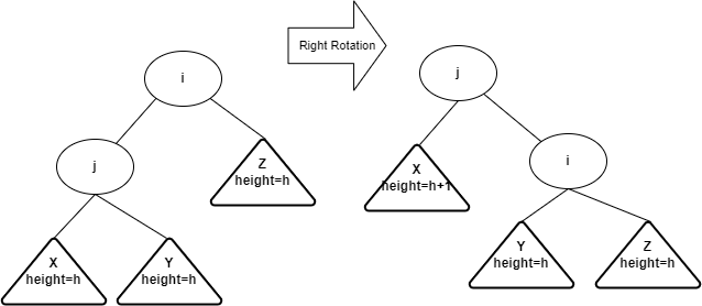
Single right rotation

Idea: after inserting into the subtree X, the tree becomes imbalanced at node j. You can do a single right rotation at node j to rebalance the tree. In the result tree, j will take the place of i

Algorithm

rotateRight(T, v) {
  // T: a BST tree
  // v: the node to be rotated
  Node y = v.left; // y cannot be null
  v.left = y.right;
  if (y.right != null) {
    y.right.parent = v;
  }
  if (v.parent == null) {
    T.root = y;
  } else {
    if (v == v.parent.left) {
      v.parent.left = y;
    } else {
      v.parent.right = y;
    }
  }
  y.right = v;
  v.parent = y;
}

Single right rotation

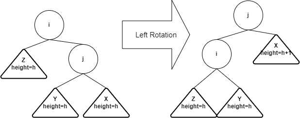
Idea: after inserting into the subtree X, the tree becomes imbalanced at node j. You can do a single left rotation at node j to rebalance the tree. In the result tree, j will take the place if i

Algorithm

rotateRight(T, v) {
  // T: a BST tree
  // v: the node to be rotated
  Node y = v.right; // y cannot be null
  v.right = y.left;
  if (y.left != null) {
    y.left.parent = v;
  }
  if (v.parent == null) {
    T.root = y;
  } else {
    if (v == v.parent.left) {
      v.parent.left = y;
    } else {
      v.parent.right = y;
    }
  }
  y.left = v;
  v.parent = y;
}

Lecture 19 2022/03/09

BST rotation
- Inside cases: double rotation
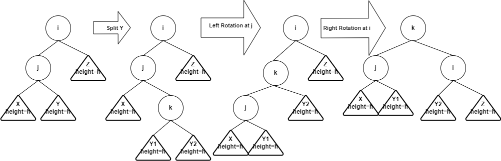
  - Left-right rotation
    - Idea: after inserting into the subtree Y, the tree becomes imbalanced at i. You first split subtree Y into two subtrees with each has height h, then do left rotation at node j, and then do right rotation at node i
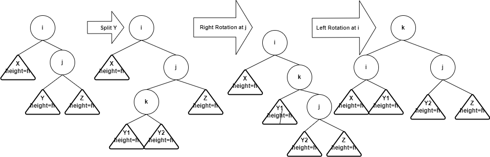
  - Right-left rotation
    - Idea: after inserting into the subtree Y, the tree becomes imbalanced at i. You first split subtree Y into two subtrees with each has height h, then do left rotation at node j, and then do left rotation at node i

Lecture 20 2022/03/10

AVL trees
- Discovered in 1962 by two Russian mathematicians
- Properties
  - BST
  - For every node in the tree the height of the left and right subtree differ by at most 1
- Algorithm
  - Search, insert, and delete as in a BST
  - After each insertion/deletion: if height of left and right subtree differ by more than 1, restore AVL property
- Balance factor
  - An AVL tree has balance factor calculated at every node
    - BF(node) = height(node.left) - height(node.right)
    - If BF(root) > 0, then the tree if left heavy
    - If BF(root) < 0, then the tree is right heavy
    - If abs(BF(root)) >= 2, then we should do rotations to restore AVL property
AVL tree insertion
- Procedures
  - Insert the new key as a new leaf just as in ordinary BST
  - Trace the path from the new leaf towards the root
  - For each node encountered calculate the balance factor
  - If the balance factor is 2 or -2, balance the tree
- For insertion, once you perform a rotation at a node v, no need to perform any rotation at ancestors of v
- Determine how to rotate after insertion
  - If v.bf < -1
    - If v.right.bf > 0: right rotate at v.right, then left rotate at v
    - IF v.right.bf < 0: left rotate at v
  - If v.bf > 1
    - If v.left.bf < 0: left rotate at v.left, then right rotate at v
    - If v.left.bf > 0: right rotate at v
AVL tree deletion
- Perform BST deletion first
- If node v is deleted, trace the path from v.parent to root, check and rotate each imbalanced node
AVL tree runtime analysis
- Search, insertion, deletion are all guaranteed to be \(O(logN)\)
Splay trees
- Splay tree is invented by Daniel Sleator and Robert Tarjan in 1983
- Splay trees are self-balancing binary search tree with additional property that recently accessed elements are quick to access again (the idea of locality)
- Splay trees do not store balance factor, they are usually nicely balanced, but height can potentially be N - 1
- Basic operations: search, insertion and deletion in amortized \(O(logN)\) time. \(O(N)\) operations can occur, but splaying makes them infrequent
- Splay tree rotations
  - If the target node X is the root of a splay tree, then no rotation is involved
  - If the target X is the child of root, then single rotation is needed. A single rotation, either left or right, is called zig
  - If the target node X has a parent P, and a grandparent G, then double rotation is involved. The double rotation, either RL rotation, or LR rotation, is called zig-zag
- Splay tree search
  - Like BST search
  - Let X be the node where the search ends (succeed or not)
  - Take node X and splay up to the root of the tree using a sequence of rotations
- Insert X
  - Like BST insert
  - Splay X to the root
- Delete X
  - First splay X to the root, and remove
  - If two subtrees remain, find the largest one from the left subtree and let it the be the new root
  - If one subtree remain, let the root of the subtree be the root of the tree
  - If no nodes remain, let the root be null
- Find max and min
  - Like BST
  - Once find the max/min, splay it to the root
- Disadvantage of splay tree
  - Amortized \(O(logN)\), it can be linear
  - For each operation, splay is needed, so there is computational overhead in maintaining a splay tree

Lecture 21 2022/03/16

Searching
- Organization and retrieval of information is at the heart of most computer applications, and searching is the most frequently performed task
- If an array is not sorted, then search is \(O(N)\), if an array is sorted, then binary search is \(O(logN)\)
Hash table ideas
- Hashing is a technique used for performing insertion, deletion, and search in constant average time
- The data structure used is the hash table
- Hash table operations: insert(T, x), delete(T, x), search(T, x)
- A table is simply another term for an array, it has several fields, to find an entry in the table, you only need to know the content of one of the fields(key, the key uniquely identifies an entry)
Direct addressing table
- Direct address tables are ordinary arrays
- Elements whose key is k obtained by indexing into the kth position of the array (if the maximum element in the table is n, then the length of a direct address table is also n)
- Insert, delete, search can be implemented to take \(O(1)\) time
- Disadvantages
  - The size of direct-address table is large
  - There could be a lot of empty space in direct address table
Hash table
- The ideal hash table is an array of some fixed size, containing items, and the operations are \(O(1)\) on average
- Hash function: a hash function transforms a key k into a number that is used as an index in an array to locate the desired location
  - An element with k hashes to slot h(k), where h(k) is the hash value of key k
  - Hash function should be simple to compute, any two distinct keys should get different cells
- Division method: h(k) = k % m, where m is the size of the table
- Issues with hashing
  - Decide what to do when two keys hash to the same value
  - Choose a good hash function
  - Choose the size of the table

Lecture 22 2022/03/17

Collision
- Collision: different keys mapped onto the same hash value
- Design a good hash function will minimize the number of collisions that occcur, but they will still happen, there are two basic collision resolution techniques
- Chaining
  - Store all elements that hash to the same slot in a linked list
  - Store a pointer to the head of the linked list in the hash table slot
  - Invented by H.P. Luhn in 1953
  - Operations
    - insert(T, x): insert x at the head of list T[h(x.key)]
    - search(T, x): search for an element with key k in list T[h(k)]
    - delete(T, x): delete x from the list T[h(x.key)]
  - Chaining is used when we cannot predict the number of records in advance, thus the choice of the size of the table depends on available memory
  - Recommendations of table size m:
    - m ~= 0.1 * n
    - m ~= n
- Open addressing
  - All elements stored in hash table itself
  - When collision occur, use a systematic procedure to store elements in free slots of the table
  - Invented by Ershov and Peterson in 1957 independently
  - If collision occurs, use this formula to do probing: h(k) = (hash(k) + f(i)) % m, where h(k) is the index in the table indicating where to insert k, hash(k) is the hash function of k, f(i) is the collision resolution function with i = 0, 1, ..., m-1, which means we start from hash(k) and try each i to find if h(k) is available, m is the size of the hash table
  - Different collision resolution functions
    - Linear probing: f(i) = i
    - Quadratic probing: f(i) = i^2
    - Double hashing: f(i) = i * hash2(k)
  - Linear probing
    - Insert
      1
      2
      3
      4
      5
      6
      7
      8
      9
      10
      11
      insert(T, k)
      i = 0
      repeat
      j = h(k, i)
      if T[j] = NIL then
      T[j] = k
      return j
      else
      i = i + 1
      until i = m
      error 'hash table overflow'
    - Search
      1
      2
      3
      4
      5
      6
      7
      8
      9
      10
      search(T, k)
      i = 0
      repeat
      j = h(k, i)
      if T[j] = k then
      return j
      else
      i = i + 1
      until T[j] = NIL or i = m
      return NIL
    - Delete is more difficult
      - If we delete a key from slot h(k), we cannot mark the slot NIL, because there maybe other probing slots based on this slot
      - We need to mark the slot with a special value, modify search so that it keeps on looking when it sees the special value, insert would treat the slot with a special value as empty slot, so a new value can be added

Lecture 23 2022/03/21

Clustering
- Primary Clustering: many consecutive elements form groups and it takes time to find a free slot or to search for an element
- Secondary Clustering: two records only have the same collision chain if their initial position is the same
- Linear probing has primary clustering problem
- Quadratic probing has secondary probing problem
Quadratic probing
- Hash function: h(k) = (hash(k) + f(i)^2) % m
- Problems: if the initial position is the same, then the collision chain will be the same
Double hashing:
- Hash function: h(k) = (hash1(k) + i * hash2(k)) % m
- A popular choice of hash2(k): hash2(k) = R - (k % R), where R is a primer number that is smaller than the size of the table
Cuckoo hashing
- Invented by Pagh and Rodler in 2001
- Idea: when we insert k1, if k2 occupies the slot, we kick it out and find k2 a new slot
- Collision strategy
  - Each hash table has a hash function h1 and h2
  - We prefer h1, but if we must move, we use h2
- Cuckoo hashing guarantees \(O(1)\) search and \(O(1)\) insert
Load factor
- Def: given a hash table T with m slots that stores n elements, load factor \(\alpha = n / m\)
- Hash with chaining: load factor can be greater than 1
- Hash with open addressing: load factor is \(0 \leq \alpha \leq 1\)
- If the load factor is high, then it's likely that there are collisions, if the load factor is low, then there are many empty slots
- If the load factor exceeds certain criteria value, then we need to do rehashing, which is an \(O(N)\) operation

Lecture 24 2022/03/23

Hash function
- A good hash function should
  - Be easy and quick to compute
  - Achieve an even distribution of the key values that actually occur across the index range supported by the table
  - Minimal number of collision
- Some hash functions
  - Middle of square: middle digits of \(k^2\)
  - Division: k % m
  - Multiplicative: the first few digits of the fractional part of k * A, where \(A = (\sqrt(5) - 1) / 2\)
  - Truncation or folding
  - String hash function: \(h(s) = s(k-1)p^{k-1} + s(1)p + s(0)\)
Sorting
- Introduction
  - \(O(N^2)\) sorting: bubble sort, insertion sort, selection sort, shell sort
  - \(O(NlogN)\) sorting: merge sort, heap sort, quick sort
  - \(O(N)\) sorting: counting sort, radix sort, bucket sort

Bubble sort

Oldest and simplest sorting algorithm
Idea: large values bubble to the end of the list while smaller values sink towards the beginning of the list
Algorithm
- Compare every pair of adjacent items, swap if necessary
- Repeat this process until no swap is made in one pass

Java implementation

public void bubbleSort(int[] a) {
  int n = a.length;
  for (int i = 0; i < n - 1; i++) {
    for (int j = 0; j < n - i - 1; j++) {
      if (a[j] > a[j + 1]) {
        int tmp = a[j + 1];
        a[j + 1] = a[j];
        a[j] = tmp;
      }
    }
  }
}

public void bubbleSort(int[] a) {
  boolean disSwap = true;
  while (disSwap) {
    disSwap = false;
    for (int i = 0; i < a.length - 1; i++) {
      if (a[i] > a[i + 1]) {
        int tmp = a[i + 1];
        a[i + 1] = a[i];
        a[i] = tmp;
        disSwap = true;
      }
    }
  }
}

Run time:
- Worst case: \(O(N^2)\)
- Best case: when sorted, \(O(N)\)
In-place: yes
Stable: yes, only swap when A[j] > A[j + 1]

Lecture 25 2022/03/24

Insertion sort

Idea: Start with an empty left part, remove one item from the right, insert it into the correct position in the left part

Java implementation

public void insertionSort(int[] a) {
  int n = a.length;
  for (int i = 1; i < n; i++) {
    int key = a[i];
    int j = i - 1;
    while(j >= 0 && a[j] > key) {
      a[j + 1] = a[j];
      j = j - 1;
    }
    a[j + 1] = key;
  }
}

Run time
- Worst case: \(O(N^2)\)
- Best case: \(O(N)\)
In-place: yes
Stable: yes, only swap when A[j] > key

Selection sort

Idea: select the smallest unsorted item in the list, swap it with the value in the first position, repeat the steps for the remainder of the list

Java implementation

public void selectionSort(int[] a) {
  int n = a.length;
  for (int i = 0; i < n - 1; i++) {
    int min = i;
    for (int j = i + 1; j < n; j++) {
      if(a[j] < a[min]) {
        min = j;
      }
    }
    int tmp = a[i];
    a[i] = a[min];
    a[min] = tmp;
  }
}

Runtime
- Worst case: \(O(N^2)\)
- Best case: \(O(N^2)\)
In-place: yes
Stable: yes, change min index only when a[j] < a[min]

Shell sort

More efficient than bubble sort, insertion sort and selection sort
A variation of the insertion sort
It compares elements that are distant rather than adjacent elements in an array or list
We can choose distant elements using gap size, gap size is one half of the length of the array and halved until each item is compared with its neighbor
Idea
- Divide array to be sorted into some number of sub-arrays
- Sort each of the sub-arrays using insertion sort
- Repeat until the length of sub-arrays being sorted is one

Java implementation

public void shellSort(int[] arr) {
  int n = arr.length;
  for (int gap = n / 2; gap > 0; gap /= 2) {
    for (int i = gap; i < n; i++) {
      int key = arr[gap];
      int j = i;
      while (j >= gap && arr[j] > key) {
        arr[j + gap] = arr[j];
        j = j - gap;
      }
      arr[j + gap] = key;
    }
  }
}

It has been proven that the gap size should not be a power of 2, use prime numbers or odd numbers instead
Runtime
- Worst case: \(O(N^2)\)
- Best case: \(O(N)\)
In-place: yes
Stable: no, shell sort uses gap intervals, so it may change the relative order of equal elements

Lecture 26 2022/03/28

Merge sort

It's invented by Neumann in 1945
It is a divide and conquer algorithm
Idea
- Divide the array into two equal-length sub-arrays
- Conquer by recursively sorting the two sub-arrays
- Combine by merging the two sorted sub-arrays to produce a single sorted array

Java implementation

private void merge(int[] arr, int lo, int mid, int hi) {
  int n1 = mid - lo + 1;
  int n2 = hi - mid;
  int[] L = new int[n1]; // L is arr[lo, ..., mid]
  int[] R = new int[n2]; // R is arr[mid + 1, ..., hi]
  for (int i = 0; i < n1; i++) {
    L[i] = arr[lo + i];
  }
  for (int j = 0; j < n2; j++) {
    R[j] = arr[mid + 1 + j];
  }
  int i = 0;
  int j = 0;
  int k = lo;
  while (i < n1 && j < n2) {
    if (L[i] <= R[j]) {
      arr[k] = L[i];
      i += 1;
    } else {
      arr[k] = R[j];
      j += 1;
    }
    k += 1;
  }
  while (i < n1) {
    arr[k] = L[i];
    i += 1;
    k += 1;
  }
  while (j < n2) {
    arr[k] = R[j];
    j += 1;
    k += 1;
  }
}

private void mergeSortHelper(int[] arr, int lo, int hi) {
  if (lo >= hi) {
    return;
  }
  int mid = lo + (hi - lo) / 2;
  mergeSortHelper(arr, lo, mid);
  mergeSortHelper(arr, mid + 1 , hi);
  merge(arr, lo, mid, hi);
}

public void mergeSort(int[] arr) {
  int n = arr.length;
  mergeSortHelper(arr, 0, n - 1);
}

Runtime
- Worst case: \(O(NlogN)\)
- Best case: \(O(NlogN)\)
In-place: no
Stable: yes

Recurrence relation
- Methods
  - Iterative
  - Recursion tree method
  - Master theorem method
- Recursion tree method
  - Example 1: \(T(n) = 2 * T(n/2) + O(n)\): \(T(n) = n + ... + n = n * logn\)
  - Example 2: \(T(n) = T(n/4) + T(n/2) + n^2\): \(T(n) = n^2 * \sum\limits_{i = 0}^{k}(\frac{5}{16})^i < n^2 * \sum\limits_{i = 0} ^{\infty}(\frac{5}{16})^i = \frac{16 n^2}{11}\)
  - Example 3: \(T(n) = 3 T(n/4) + cn^2\): \(T(n) < \frac{16n^2}{13}\)

Lecture 27 2022/03/30

Quick sort

Idea: sort array A[p, ..., q]
- Divide: partition the array into two sub-arrays around an element called pivot x, (A[p, ..., x - 1], A[x + 1, ..., q]). Elements in the lower sub-array are less than or equal to x, elements in the upper sub-array are greater than or equal to x
- Conquer: recursively sort the two sub-arrays
- Combine: trivial

Java implementation

private void partition(int[] arr, int lo, int hi) {
  int pivot = arr[lo];
  // i is the index of rightmost item that is <= pivot
  int i = lo;
  for (int j = lo + 1; j <= hi; j++) {
    if (arr[j] <= pivot) {
      i += 1; 
      // arr[i] the first item > pivot, a[j] <= pivot, so we swap the two
      // after swap, i again is the index of rightmost item that is <= pivot
      int tmp = arr[i];
      arr[i] = arr[j];
      arr[j] = tmp;
    }
  }
  arr[lo] = arr[i];
  arr[i] = pivot;
  return i;
}

private void quickSortInner(int[] arr, int lo, int hi) {
  if (lo >= hi) {
    return;
  }
  int x = partition(arr, lo, hi);
  quickSortInner(arr, lo, x - 1);
  quickSortInner(arr, x + 1, hi);
}

public void quickSort(int[] arr) {
  int n = arr.length;
  quickSortInner(arr, 0, n - 1);
}

Runtime
- Worst case: \(O(N^2)\)
- Best case: \(O(NlogN)\)
In-place: yes
Stable: no, it swaps elements according to the pivot's position

Lecture 28 2022/03/31

Randomized quick sort
- Motivation: we don't want quick sort to be \(O(N^2)\)
- Idea: partition around a random element
  - Running time is independent of the input order
  - No assumptions need to be made about the input distribution
  - The worst case is determined only by the output of a random-number generator
- Pick a random element as the pivot

Sorting in linear time

Comparison-based sorting algorithms:
- Merge sort and heap sort achieve \(O(NlogN)\) time in worst case
- Quick sort achieves \(O(NlogN)\) time on average
Non comparison-based linear time sorting algorithms:
- Example: counting sort, radix sort, and bucket sort

Counting sort

Algorithm

countingSort(A, B, k)
  # Input: A[1...n], where A[i] in {1, 2, ..., k}
  # Output: B[1...n], B is sorted
  
  Initialize C[0...k]
  for i <- 0 to k do
    C[i] <- 0
  for j <- 1 to size of A do
    C[A[j]] <- C[A[j]] + 1  # Calculate the frequency of items in array A
  for i <- 1 to k do
    C[i] <- C[i] + C[i - 1] # Cumulative frequency, also the last index of an item in the sorted array
  for j <- size of A downto 1 do
    B[C[A[j]]] <- A[j]
    C[A[j]] <- C[A[j]] - 1

Stable: yes
Complexity: \(O(N + k)\)

Lecture 29 2022/04/04

Heap

Introduction
- A heap is a tree-like data structure that can be implemented as an array
- Each node of the tree corresponds to an element of the array and every node must satisfy the heap properties
- There are different variants of heap: 2-3 heap, beap, Fibonacci heap, d-ary heap, binary heap

Binary heap

A binary heap is a complete binary tree that satisfies the heap property
- Let v and u be nodes of a heap, such that u is a child of v
- If v.data >= u.data, we have a max heap
- If v.data <= u.data, we have a min heap
- Min heap: a complete binary tree where the key of each node is less than the keys of its children
- Max heap: a complete binary tree where the key of each node is greater than the keys of tis children
Array index of a binary heap
- When the array of a binary heap is 1-indexed, if node v is at index n, its left child is at index 2 * n, its right child is at index 2 * n + 1, its parent is at index [n / 2]
- When the array of a binary heap is 0-indexed, if node v is at index n, its left child is at index 2 * n + 1, its right child is at index 2 * n + 2, its parent is at index [(n - 1) / 2]
Basic heap operations
- Build-max-heap/build-min-heap: create a max-heap/min-heap from an unordered array
- Insert a node: new nodes are always inserted at the bottom level from left to right
- Delete a node: nodes are removed from the bottom level from right to left
- Heapsort: sort an array in place
- Heapify: the key to maintain the heap property
  - Heapify up/percolate up
  - Heapify down/percolate down

Implementation

Heapify down for max heap, time complexity: \(O(logN)\)

public void heapifyDown(int[] A, int k) {
  // A is an array of size n + 1 if the heap contains n elements, because
  // ideally we want an 1-indexed array but there is no such thing in Java 
  int n = A.length;
  int left = 2 * k;
  int right = 2 * k + 1;
  int largest = k;
  if (left < n && A[left] > A[largest]) {
    largest = left;
  }
  if (right < n && A[right] > A[largest]) {
    largest = right;
  }
  if (largest != k) {
    int tmp = A[k];
    A[k] = A[largest];
    A[largest] = tmp;
    heapifyDown(A, largest);
  }
}

Heapify up for max heap, time complexity: \(O(logN)\)

public void heapifyUp(int[] A, int k) {
  while (k > 1 && A[i] > A[i / 2]) {
    int tmp = A[k];
    A[k] = A[k / 2];
    A[k / 2] = tmp;
    k = k / 2;
  }
}

Lecture 30 2022/04/06

Heap

Height: since a heap is a complete binary tree, the height of a heap of N elements is \(logN\)
Basic operations on heaps run in proportional to the height, \(O(logN)\)

Build a max heap, time complexity: \(O(NlogN)\)

public void buildMaxHeap(int[] A) {
  int len = A.length;
  for (int i = (len - 1) / 2; i >= 1; i /= 2) {
    heapifyDown(A, i);
  }
}

In order to build a min heap, the logic is the same, the only modification is in the hepifyDown method that we need to swap the element with its smallest child when necessary

Heapsort

Goal: sort an array using heap implementation
Idea:
- Build a max heap from an array
- Swap the root with the last element in the array
- Decrease the size of the heap by 1
- Call heapify down on the new root
- Repeat this process until only one node remains in the heap

Implementation

public void heapSort(int[] A) {
  buildMaxHeap(A);
  int n = A.length;
  for (int i = n - 1; i >= 2; i--) {
    int tmp = A[1];
    A[1] = A[i];
    A[i] = tmp;
    heap.size -= 1;
    heapifyDown(A, 1);
  }
}

Time complexity: \(O(NlogN)\)
In place: yes
Stable: no

Priority Queue
- A priority queue is a data structure for maintaining a set of elements with priorities, the key withe the highest/lowest priority is extracted first
- Max priority queue operations
  - Insert(A, x): insert the element x in A, x has a priority with it
  - Extract-Max(A): removes and returns the element of A with the largest key
  - Maximum(A): returns the element of A with the largest key
  - Increase-key(A, x, k): increase the value of element's priority to the new value k, which is assumed to be at least as large as x's current priority
- Implementation
  1
  2
  3
  4
  // O(1) operation
  public int getMax(A) {
  return A[1];
  }
  1
  2
  3
  4
  5
  6
  7
  8
  // O(logN) operation
  public int extractMax(A) {
  int max = A[1];
  A[1] = A[A.length - 1];
  A.heapSize -= 1;
  heapifyDown(A, 1);
  return max;
  }
  1
  2
  3
  4
  5
  // O(logN) operation
  public void increaseKey(A, i, key) {
  A[i] = key;
  heapifyUp(A, i);
  }
  1
  2
  3
  4
  5
  6
  // O(logN) operation
  public void insert(A, key) {
  A.heapSize += 1;
  A[A.heapSize] = key;
  increaseKey(A, A.heapSize, key);
  }

Lecture 31 2022/04/07

Graph
- A graph models a set of connections
- A graph G = (V, E) consists of
  - A finite set V of vertices, |V| is called the order of a graph
  - A finite set E of edges, |E| is called the size of a graph, each edge is a pair (u, v) where u, v \(\in\) V
- Applications of Graphs
  - Road maps
  - Chemical structures
  - Games/ puzzles
  - Computer networks
  - Web links
- Edge types
  - Direction
    - Directed edge: ordered pair of vertices (u, v), u is called the origin, v is called the destination
    - Undirected edge: unordered pair of vertices (u, v)
  - Weight
    - Weighted edge
    - Unweighted edge
  - A graph may be directed or undirected, weighted or unweighted
- Terminology
  - Adjacent vertices: two vertices connected by an edge
  - Degree of a vertex: the number of edges starting or ending at that vertex
    - In-degree: the number of edges ending at a vertex
    - Out-degree: the number of edges starting at a vertex
  - Path: a sequence of edges
  - Length of a path: the number of edges on a path
  - Simple path: a path where all its vertices and edges are distinct
  - Cycle: a path beginning and ending at the same vertex
  - Simple cycle: a simple cycle is a cycle which does not pass through any vertex more than once
  - Loop: an edge whose endpoints are the same vertex

Lecture 32 2022/04/11

Implementing graphs
- Data structure for vertices
  - Hash table (generally preferred)
  - Array
  - List
  - Binary search tree
- Data structures for edges
  - Adjacency list
  - Adjacency matrix
- Adjacency list
  - Consists of an array of length |V|, each position in the list is for a vertex in V
  - For the position associated with vertex u in the array, the adjacency list consists of all vertices v such that there is an edge (u, v) \(\in\) E
- Adjacency matrix
  - It consists of an |V| * |V| binary matrix M
  - If the graph is directed, \(M[i][j] = 1 \iff (i, j) \in E\)
  - If the graph is undirected, \(M[i][j] = M[j][i] = 1 \iff (i, j) \in E\)
- The time complexity of graph algorithms are often expressed in |E| and |V|

Graph traversal

Two kinds of graph traversal algorithm
- Breadth-first search (BFS)
- Depth-first search (DFS)

BFS

BFS is the archetype for many graph algorithms: Dijkstra's shortest path algorithm, Prim's minimum spanning tree algorithm
Idea: given a graph G and a source vertex s, BFS systemically explores the edge of G to discover every vertex that is a reachable from s

Implementation

public void BFS(Graph G, int s) {
  // you can also use boolean[] visited = new boolean[G.V()]
  int[] dist = new int[G.V()];
  for (int i = 0; i < G.V(); i++) {
    dist[i] = Integer.MAX_VALUE;
  }
  dist[s] = 0;
  Queue<Integer> queue = new Queue<Integer>();
  queue.enqueue(s);
  while (!queue.isEmpty()) {
    int u = queue.dequeue();
    System.out.println(u);
    for (int v: G.adj(u)) {
      // if vertex v has not been visited
      if (dist[v] == Integer.MAX_VALUE) {
        dist[v] = dist[u] + 1;
        queue.enqueue(v);
      }
    }
  }
}

Time complexity: \(O(V + E)\)

Lecture 33 2022/04/13

Shortest path problem

Use a weighted graph
The weight of a path is the sum of the weights of its edges
Let \(\{w(p): u \rightarrow v\}\) be the set of the weights of all paths from u to v, if the set has a minimum, we call the minimum the shortest path weight from u to v, denote \(\delta(u, v)\). If the set does not has a minimum, denote \(\delta(u, v) = \infty\) (If u and v are not connected, or if there is a cycle with negative weight in the path from u to v)

Single source shortest path problem with Dijkstra's algorithm

Description: find a shortest path from a given source vertex s to each of the vertices in the graph
Assumptions
- Directed graph
- All edges must have nonnegative weights
- Connected graph

Implementation

public int[] dijkstra(G, int src) {
  int[] dist = new int[G.V()];
  // prev[i] is the previous vertex of vertex i in the shortest path from src to i
  // path from src to i is prev[i] -> prev[prev[i]] -> ... -> src
  int[] prev = new int[G.V()];
  for (int i = 0; i < G.V(); i++) {
    dist[i] = Integer.MAX_VALUE;
    prev[i] = -1;
  }
  dist[src] = 0;
  prev[i] = -1;
  PriorityQueue<Integer> pq = new PriorityQueue<Integer>(G.V(), new Comparator<Integer>() {
    public int compare(Integer a, Integer b) {
      return dist[a] - dist[b];
    }
  });
  for (int i = 0; i < G.V(); i++) {
    pq.enqueue(i, dist[i]);
  }
  while (pq.isEmpty()) {
    int u = pq.remove();
    for(int v: G.adj(u)) {
      if (dist[v] > dist[u] + G.weight(u, v)) {
        dist[v] = dist[u] + G.weight(u, v);
        prev[v] = u;
      }
    }
  }
  return dist;
}

Time complexity: \(O((V + E)logV)\)

Lecture 34 2022/04/14

Depth-first search

Problems solved by DFS
- Testing whether a graph is connected
- Computing a path between two vertices or equivalently reporting that no such path exists
- Compute a cycle or equivalently reporting the no such cycle exists

Algorithm

DFS(V, E)
  for each u in V do
    u.color = WHITE
  time = 0
  for each u in V do
    if u.color = WHITE then
      DFS-VISIT(u)
DFS-VISIT(u)
  u.color = GRAY
  time = time + 1
  u.i = time
  for each v in Adj(u) do
    if v.color = WHITE then
      DFS-VISIT(v)
  u.color = BLACK
  time = time + 1
  u.f = time

Time complexity: \(O(V + E)\)

Edge classification
- The edge in DFS can be classified into four types: tree edge, back edge, forward edge and cross edge
- Consider edge (u, v)
  - If v is visited for the first time, then (u, v) is a tree edge
  - If v is an ancestor of u, then (u, v) is a back edge
  - If v is a descendant of u, then (u, v) is a forward edge
  - If u is neither an ancestor nor a descendant of v, then (u, v) is a cross edge

Lecture 35 2022/04/25

Edge classification
- Facts
  - If G is undirected, then there are only tree and back edges
  - If G is DAG \(\rightleftarrows\) DFS on G yields no back edges
- Cycle detection
  - A directed graph G contains a cycle if and only if a DFS of G yields a back edge
Topological sort
- A topological sort of a DAG is a linear ordering of all its vertices such that if DAG contains an edge (u, v), then u appears before v in ordering
- Algorithm
  1
  2
  3
  4
  TOPOLOGICAL-SORT(G)
  call DFS(G) to compute the finishing times of each vertex
  when each vertex is finished, insert it onto the front of a linked list
  return the linked list
- Performance
  - Time complexity: \(O(V + E)\)
  - Space complexity: \(O(V + E)\)

Lecture 36 2022/04/27

Graph connectivity
- Definition
  - Connected vertices: in an undirected graph G, two vertices u and v are called connected if G contains a path from u to v. Otherwise, they are called disconnected
  - Connected graph: a undirected graph is said to be connected if every pair of vertices in the graph is connected. Otherwise, the graph is disconnected
    - A graph consisting of one vertex is connected
  - Connected component: if a undirected graph is not connected, then each piece is called a connected component
    - If a graph is connected, then the thole graph is one single connected component
  - Connectivity for directed graph
    - Strongly connected: if there s a path in each direction between each pair of vertices of a directed graph, then it is strongly connected
    - If a graph is not strongly connected, then it is weakly connected
- Strongly connected components
  - A classical application of DFS is to decomposing a directed graph into strongly connected components
  - Graph transpose/reverse: given a graph \(G = (V, E)\), its transpose is \(G^{T} = (V, E^{T})\), where \(E^{T} = \{(u, v) | (v, u) \in E \}\)
  - Algorithm
    1
    2
    3
    call DFS(G) to compute finished time u.f for each v in V
    call DFS(G^T), consider the nodes in order of decreasing u.f
    output the strongly connected components
Minimum spanning tree
- Definition
  - Spanning tree: a spanning tree is a subgraph that consists all the vertices and is a tree
  - Minimum spanning tree: a spanning tree that has minimal total weight of its edges is called a minimum spanning tree
- Algorithms: both greedy algorithms
  - Prim's algorithm
  - Kruskal's algorithm
P vs NP
- P: the class of all problems that have an algorithm that can be computed in polynomial time
- NP: the class of all problems that can be verified in polynomial time but may take an exponential time to solve
  - Some NP problems are P problems and can be solved in polynomial time or less
  - The hardest NP problems are NP-complete, which have never been shown to be solvable in polynomial time: e.g. the traveling salesman problem, the hamiltonian cycle problem
- The problem is whether P = NP

Operation	Average	Worst
Search	\(O(logn)\)	\(O(n)\)
Insert	\(O(logn)\)	\(O(n)\)
Delete	\(O(logn)\)	\(O(n)\)