Course Name: Introduction to Machine Learning

Instructor: Professor Lawrence Carin, Professor David Carlson, Timothy Dunn, Kevin Liang

Week 1

Logistic Regression
- Why Machine Learning is Exciting
  - DL in the analysis of images: the ImageNet Challenge: evaluates algorithms for object detection and image classification at large scale
  - DL in games:solve a complex sequential problem
- What is Machine Learning
  - In ML we give the machine data, and teach them to build models and make predictions
  - Terminology: x: data/feature, y:outcome, training data
- Logistic Regression
  - Process: training set => mathematical model => learned parameters => make predictions on new data
  - Linear predictive model
    - Data: \(x_{i1}, x_{i2},..., x_{iM}\), \(y_1, y_2, ..., y_M\)
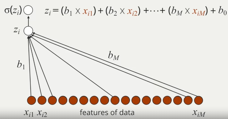
    - Model: \(z_i = b_0 + b_1 x_{i1} + b_2 x_{i2} + ... + b_M x_{iM}\), the parameters tell how important the data variables are to the prediction
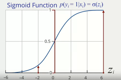
    - Sigmoid function: \(p(y_i = 1|x_i) = \sigma(z_i)\), the sigmoid function convert predictions to a probabilistic perspective
- Interpretation of Logistic Regression
  - Digit recognition problem on the MNIST Data Set: decompose the handwritten number figures into pixels and convert the color into a number for each pixel, then regard the training set as the set of numbers for each figure, run a logistic regression on the training set and use the result to distinguish which number is written
- Motivation for Multilayer Perceptron
  - Linear classifiers can only represent limited relationships, we often want to use a classifier thant can handle non-linearities
Multilayer Perceptron
- Concepts
  - Logistic regression: M features of data => a single filter => probability of a particular outcome
  - Multilayer perceptron: M features of data => K filters => probability of K latent processes/features => probability of a particular outcome
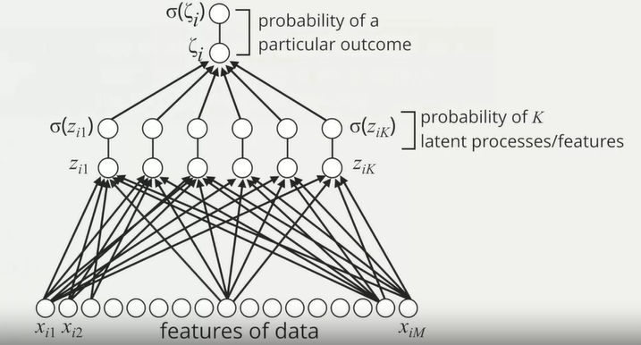
  - The multilayer perceptron can be viewed as logistic regression on K latent features, rather than directly on the M components of raw data
- Math Model
  
  \(z_{i1} = b_{01} + b_{11} x_{i1} + b_{21} x_{i2} + ... + b_{M1} x_{iM}\), \(\; p(y_i = 1|x_i, b_1) = \sigma(z_{i1})\)
  
  \(z_{i2} = b_{02} + b_{12} x_{i1} + b_{22} x_{i2} + ... + b_{M2} x_{iM}\), \(\; p(y_i = 1|x_i, b_2) = \sigma(z_{i2})\)
  
  \(\qquad \qquad \qquad \qquad \qquad \vdots\)
  
  \(z_{iK} = b_{0K} + b_{1K} x_{i1} + b_{2K} x_{i2} + ... + b_{MK} x_{iM}\), \(\; p(y_i = 1|x_i, b_K) = \sigma(z_{iK})\)
  
  \(\zeta_is = c_0 + c_1 \sigma(z_{i1}) + c_2 \sigma(z_{i2}) + ... + c_K \sigma(z_{iK})\)
- Deep Learning
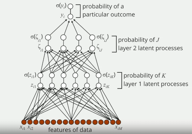
  - Deep learning is a form of machine learning where a model has multiple layers of latent processes
- Multilayer Perceptron: Neural Network
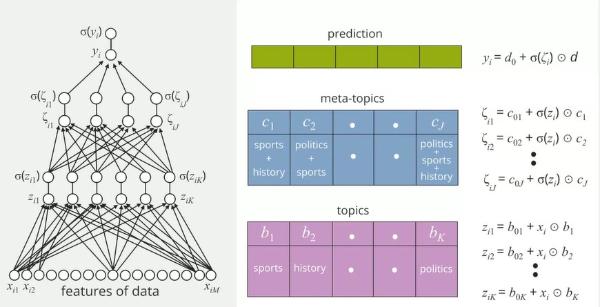
- Transfer Learning
  - Considering multiple likes and dislikes
    - The first-two layers look for topics and meta-topics, and thus can be used in models of multiple people, parameters "transferred" across all data, documents, and people
    - The top layer characterizes specific people, parameters are different for each people
- Model Selection
  - Bias-Variance trade-off
    - Variance: the more complex the model is, the bigger variance it has. The variation of outputs for different inputs of a model is the variance of the model
    - Bias: the simpler the model is, the more biased it is
    - Logistic regression: bigger bias, smaller variance
    - Multilayer perceptron: smaller bias, bigger variance
  - Logistic regression results in a linear classifier, while multilayer perceptron results in a non-linear classifier
- History of Neural Networks
  - Seasons of Neural Networks:
    - 1960 Multilayer Perceptron(MLP) 多层感知机
    - 1986 Back Propagation 反向传播(BP算法)
    - 1989 Convolutional Neural Network(CNN) 卷积神经网络
    - 1990 - 1994 Neural Nets in the Wild: insufficient training data
    - 1995 Long Short-Term Memory(LSTM) 长短期记忆网络
    - 1998 - 2005 More Neural Nets in the Wild: not good performance
    - 2005 - 2010 Banishment: no neural network at all because of bad performance
    - 2010 Rename: Deep Learning
    - 2013 CNN + GPU(parallel computation) + ImageNet(image dataset)
    - 2015 AlphaGo: based on CNN and Reinforcement Learning
  - Occam's razor: all things being equal, the simplest solution tends to be the best one
Convolutional Neural Networks
- Hierarchical Structure of Images
  - Picture(most complex) => high-level motifs => repeated sub-structures called sub-motifs => atomic elements(simplest)
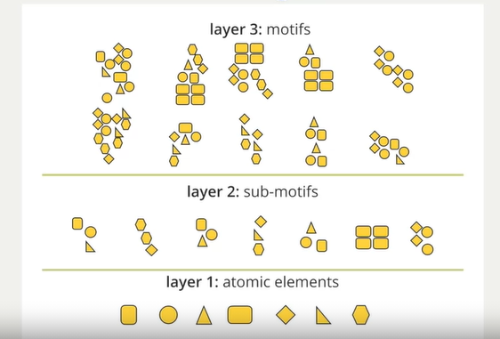
  - Structures: edges, corners, textures, shapes, ...
- Convolution Filters
  - Layer 1 Convolution: shift an atomic element to every possible location in an image, check the correlation between the atomic element and the local region, the process is the called the convolution, the correlations make a feature map. We do so for each atomic element to construct multiple feature maps
  - Layer 2 Convolution: shift combination of atomic elements to every possible location in the feature maps. Construct layer 2 feature maps in such a way.
  - Layer 3 Convolution: shift sub-motifs with layer 2 feature maps to construct layer 3 feature maps
- Convolutional Neural Network
  - CNN classifier is based on layer 3 feature maps
- CNN Math Model
  - Layer 1:
    
    \(\quad M_n = f(I_n;\phi_1, ..., \phi_K)\) where \(I_n\) represents the ith image, and \(\phi_1,..., \phi_K\) represents layer 1 filters
  - Layer 2:
    
    \(\quad L_n = f(M_n;\Psi_1, ..., \Psi_K)\) where \(M_n\) represents the ith layer 1 feature map, and \(\Psi_1,..., \Psi_K\) represents layer 2 filters
  - Layer 3:
    
    \(\quad G_n = f(L_n;\omega_1, ..., \omega_K)\) where \(L_n\) represents the ith layer 2 feature map, and \(\omega_1,..., \omega_K\) represents layer 3 filters
  - Classifier:
    
    \(\quad l_n = l(G_n;W)\)
- How the Model Learns
  - We have labeled data \(\{I_n,\; y_n\}\), where \(y_n \in \{+1,\; -1\}\)
  - Risk function of model parameters \(E(\Phi,\; \Psi,\; \Omega,\; W) = 1/N \sum {loss(y_n,\;l_n)}\)
  - Find model parameters \(\hat{\Phi},\;\hat{\Psi},\;\hat{\Omega},\;\hat{W}\) that minimize \(E(\Phi,\;\Psi,\;\Omega,\;W)\)
- Advantages of Hierarchical Model
  - Top level motifs would be learned independently if we do not use hierarchy
  - Sharing similarities allows more effective data use
  - Facts
    - Learning is manifested by taking large quantities of labeled data
    - Learning is the concept of estimating the model parameters so the predictions are consistent with true labels
Applications in the Real World
- CNN on Real Images
- Application in Use and Practice
  - Image Processing
  - DL in Games
  - Digit Recognition
- Deep Learning and Transfer Learning
  - Image analysis in radiology, ophthalmology, dermatology in medicine industry
  - DL can access massive quantities of labeled data, but this not possible or way too expensive in medicine industry, so we need transfer learning here
  - And we can sometimes even transfer parameters from models implemented in vast different areas
PyTorch Basics
- Conda commands
  - conda clean
  - conda config
  - conda create
  - conda info
  - conda install
  - conda list
  - conda remove
  - conda update
  - conda search
- For users from mainland China, you can add tsinghua channel to speed up
- Installation
  - Install some supporting dependencies: conda install h5py imageio jupyter matplotlib numpy tqdm
  - Install PyTorch: conda install pytorch torchvision cpuonly -c pytorch
- Advantages of using PyTorch
  - Library functions
  - Computational efficiency + GPU support
  - Auto-differentiation
  - Online community

Week 2

Logistic Regression as Running Example
- How Do We Define Learning?
  - Define what is performance. Given data, find the best parameters that give us the best performance with least resources used
  - Empirical risk minimization
    - A loss function defines a penalty for poor predictions
    - Want to minimize average loss: \(b^{*} = \underset{b}{\operatorname{argmin}} \frac{1}{N}\sum\limits_{i = 1}^{N} l(y_{i},\sigma(z_{i}))\)
      
      where \(b^{*}\) is the optimal parameters, \(\sigma(z_{i})\) is the predicted probability, \(y_i\) is the true label, we can use the negative log-likelihood function as the loss function, \(l(y_i, \sigma(z_i)) = -log(p(y_i|\sigma(z_i)))\).
      
      In binary classification problem, we have
      
      \[l(y,\sigma(z)) = -ylog(\sigma(z)) - (1 - y)log(1 - \sigma(z))\]
- How Do We Evaluate Our Networks?
  - We can use DL to calculate complex relationships, but models need to be validated
  - Overfitting: when the learned model increases complexity to fit the observed training data too well but not predicts well in real world
    - Increase parameters, increase error rate
    - The learned relationship is too complex for reality, so models and analyses are not generalized
  - Validating process
    - Ideal way: collecting new real-world data is useful, but it costs way too much
    - We can split existing data into separate groups, training data set, validation data set and testing data set.
      - Test set: never used to learn or fit parameter, can evaluate performance ot network, is should be used only once, reusing a test set will lead to bias
      - Validation set: used to compare which approach is best, not used to learn parameters, use repeatedly to estimate the performance, can be used to pick the best performance model
Learning via Gradient Descent
- How Do We Learn Our Network?
  - Minimize \(b^* = agrmin f(b)\) using gradient descent
    - Start with initial value \(b^0\)
    - Run series of updates to move from \(b^k\) to \(b^{k + 1}\), \(b^{k + 1} = b^{k} - a^{k} \nabla f(b^{k})\), where \(a^{k}\) is the step size
    - Repeat step 2 and step 3 until solution is good enough
- How Do We Handle Big Data?
  - Calculate the gradient requires looking at every single data point, which is unbearable
    
    \[\nabla\frac{1}{N}\sum\limits_{i = 1}^{N} l(y_{i},\sigma(z_{i})) = \frac{1}{N}\sum\limits_{i = 1}^{N} \nabla l(y_{i},\sigma(z_{i}))\]
  - We use approximations to improve calculation speed vastly \[\nabla l(y_{j},\sigma(z_{j})) \approx \frac{1}{N}\sum\limits_{i = 1}^{N} \nabla l(y_{i},\sigma(z_{i}))\]
    
    where j is a randomly picked point, this is called stochastic gradient descent. This can work because there is often redundant data
  - Minimize \(b^* = agrmin f(b)\) using stochastic gradient descent
    - Start with initial value \(b^0\)
    - Choose a random data entry j
    - Estimate gradient \(\widehat{\nabla f}(b^{k})\) by data point j
    - Iteratively update: \(b^{k + 1} = b^{k} - a^{k} \widehat{\nabla f}(b^{k})\)
    - Repeat step 2 to step 4 until solution is good enough
  - In practice, we're often going to use a mini-batch. Which means that instead of using a single data example, we're going to run a few data examples to estimate the gradient and this will reduce variance.
- Early Stopping
  - Maximizing generalization of network is mismatched with our optimization goal, because the goal of optimization is to do as well as possible on our training set. Taken overfitting into account, it may be better to stop earlier.
  - Early stopping:
    - Can check validation loss as we go
    - Instead of optimizing to convergence, optimize until validation loss stops improving(during the optimization loop, check the validation loss, stop when loss stops improving)
    - Helps save computational cost
    - Will perform better in the real world

Model Learning with PyTorch

Logistic Regression

MNIST Dataset

Prepare the data using torchvision package

from torchvision import datasets, transforms

mnist_train = datasets.MNIST(root="./datasets", train=True, transform=transforms.ToTensor(), download=True)
mnist_test = datasets.MNIST(root="./datasets", train=False, transform=transforms.ToTensor(), download=True)

Use a DataLoader to take care of shuffling and batching instead of working directly with the dataset

1 2	train_loader = torch.utils.data.DataLoader(mnist_train, batch_size=100, shuffle=True) test_loader = torch.utils.data.DataLoader(mnist_test, batch_size=100, shuffle=False)

Logistic Regression Model

The model \(Y = XW + b\), where \(Y \in \boldsymbol{R}^{m*c}\), \(X \in \boldsymbol{R}^{m*d}\), \(W \in \boldsymbol{R}^{d*c}\), \(b \in \boldsymbol{R}^{c}\)

Initialization

x = images.view(-1, 28*28)

# Randomly initialize weights W
W = torch.randn(784, 10)/np.sqrt(784)
W.requires_grad_()

# Initialize bias b as 0s
b = torch.zeros(10, requires_grad=True) 

# Linear transformation with W and b
y = torch.matmul(x, W) + b

Calculate probabilities \(p(y_{i}) = \frac{exp(y_{i})}{\sum_{j} exp(y_{j})}\)

# Option 1: Softmax to probabilities from equation
py_eq = torch.exp(y) / torch.sum(torch.exp(y), dim=1, keepdim=True)

# Option 2: Softmax to probabilities with torch.nn.functional
import torch.nn.functional as F
py = F.softmax(y, dim=1)

Cross-Entropy Loss: \(H_{y^{'}}(y) = \sum_{i}y^{'}_{i}log(y_{i})\), where \(y_{i}\) is the model predicted value, and \(y^{'}_{i}\) is the true label

# Option 1: Cross-entropy loss from equation
cross_entropy_eq = torch.mean(-torch.log(py_eq)[range(labels.shape[0]),labels])

# Option 2: cross-entropy loss with torch.nn.functional
cross_entropy = F.cross_entropy(y, labels)

The Backward Pass: update the model by changing the parameters in order to minimize the loss function

\[\theta_{t + 1} = \theta_{t} - \alpha \nabla_{\theta} \mathcal{L} \]

where \(\theta\) is the parameter(here is W and b), \(\alpha\) is the learning rate(step size), and \(\nabla_{\theta}\mathcal{L}\) is the gradient of our loss with respect to \(\theta\)
1
2
# Optimizer
optimizer = torch.optim.SGD([W,b], lr=0.1)

Model Training

To train the model, we just need repeat what we just did for more minibatches from the training set. As a recap, the steps were:

Draw a minibatch
Zero the gradients in the buffers for W and b
Perform the forward pass (compute prediction, calculate loss)

Perform the backward pass (compute gradients, perform SGD step)

# Iterate through train set minibatchs 
for images, labels in tqdm(train_loader):
    # Zero out the gradients
    optimizer.zero_grad()
    
    # Forward pass
    x = images.view(-1, 28*28)
    y = torch.matmul(x, W) + b
    cross_entropy = F.cross_entropy(y, labels)
    # Backward pass
    cross_entropy.backward()
    optimizer.step()

Testing

## Testing
correct = 0
total = len(mnist_test)

with torch.no_grad():
    # Iterate through test set minibatchs 
    for images, labels in tqdm(test_loader):
        # Forward pass
        x = images.view(-1, 28*28)
        y = torch.matmul(x, W) + b
        
        predictions = torch.argmax(y, dim=1)
        correct += torch.sum((predictions == labels).float())
    
print('Test accuracy: {}'.format(correct/total))

Week 3

Convolutional Neural Network Basics
- Motivation: Diabetic Retinopathy
  - Diabetic retinopathy classification :
    - \(sensitivity = \frac{number \; of \; true \; positives}{total \; number \; of \; positives \; in \; the \; dataset}\)
    - \(specificity = \frac{number \; of \; true \; negatives}{total \; number \; of \; negatives \; in \; the \; dataset}\)
  - DL for image analysis: TSA screening
- Breakdown of the Convolution(1D and 2D)
  - Definition: \((f * g)(t) := \int\limits_{-\infty}^{\infty}{f(\tau)g(t - \tau)d\tau}\)
  - 1D spatial convolution example:
    - \((f * g)[n] = \sum\limits_{m = - \infty}^{\infty} f[m]g[-(n+m)]\)
  - 2D spatial convolution is similar
Core Components of the Convolutional Layer
- Core elements:
  - Convolutional layers
  - Activation functions
  - Pooling layers
  - Fully connected layers
- Convolutional layers:
  - Filter size: n by n filter
  - Filter stride: if filter stride = n, then the filter moves n pixels on the image each time. The filter stride helps reduce the computational load by down-sampling the input
  - Filter number: the number of filters determine the number of unique feature detectors that operate on the inputs
- Activation functions
  - An activation function in a neural network defines how the weighted sum of the input is transformed into an output from a node or nodes in a layer of the network.
  - Both linear activation function and non-linear activation function can be used. Non-linear activation functions increase the functional capacity of the neural network. Non-linear activations examples: sigmoid function, rectified linear unit(ReLU)
- Pooling and Fully Connected Layers
  - Functions of the pooling layer
    - Reduce computational complexity
    - Combat overfitting
    - Encourage translational invariance
  - Fully Connected Layer
    - Flatten or vectorize the pooling layer
    - Each neuron in the fully connected layer has connections to all of the upstream elements in the pooling layer
    - Multiple latent fully connected layer can be built
CNN Implementations
- Training the Network
  - CNN Math model review
  - Gradient descent and stochastic gradient descent review
- Transfer Learning and Fine-Tuning
  - Transfer learning review
CNN with PyTorch
- CNN Lab
  - Fully connected layer: \(\; 𝑦=ReLU(𝑥𝑊+𝑏)\)
    
    where \(x \in \mathbb{R}^{M * C_{in}}\) is the input, \(M\) is mini-batch size, \(C_{in}\) is the dimensionality of the input. \(W \in \mathbb{R} ^{C_{in} * C_{out}}\), \(C_{out}\) is the dimensionality of the output, \(b \in \mathbb{R} ^{M * C_{out}}\), \(W\) and \(b\) are variables that we are trying to learn for our model. \(y \in \mathbb{R} ^{M * C_{out}}\) is the output.
  - Convolutional layer: \(\; 𝑦=ReLU(𝑥𝑊+𝑏)\)
    
    where \(x \in \mathbb{R}^{M * C_{in} * H_{in} * W_{in}}\) is the input, \(M\) is mini-batch size, \(C_{in}\) is the number of channels of the input, \(H_{in}\) is the height of the image, \(W_{in}\) is the width of the image. \(W \in \mathbb{R} ^{C_{in} * C_{out} *H_{k} * W_{k}}\), \(C_{out}\) is the dimensionality of the output, \(H_{k}\) is the kernel height, \(W_{k}\) is the kernel weight, \(b \in \mathbb{R} ^{M * C_{out}* H_{out} * W_{out}}\), \(W\) and \(b\) are variables that we are trying to learn for our model. \(y \in \mathbb{R} ^{M * C_{out} * H_{out} * W_{out}}\) is the output.
  - Reshaping:
    1
    2
    3
    import torch
    M = torch.zeros(4, 3)
    M2 = M.view(1, 1, 12)
  - Pooling and striding
    - Pooling: The two most common forms of pooling are max pooling and average pooling. Both reduce values within a window to a single value, on a per-feature-map basis. Max pooling takes the maximum value of the window as the output value; average pooling takes the mean.
    - Striding: While pooling is an operation done after the convolution, striding is part of the convolution operation itself.
  - Torchvision: Torchvision includes easy-to-use APIs for downloading and loading many popular vision datasets.

My Blog

Introduction to Machine Learning Notes

Week 1

Week 2

Week 3