Course Name: Algorithms, Part I
Instructor: Professor Kevin Wayne, Professor Robert Sedgewick
Books: Algorithms(4th edition)
Week 1
- Introduction
- Course Structure:
- Course Structure:
- Analysis of Algorithms
- Introduction
- Running time is the key concern
- Reasons to analyze algorithms:
- Predict performance
- Compare algorithms
- Provide guarantees
- Understand theoretical basis
- Scientific method applied to analysis of algorithms
- observe => hypothesize => predict => verify => validate
- Experiments must be reproducible, hypotheses must be falsifiable
- Observations
- Use plots to analyze algorithms:
- Standard plot:
(problem size N, running time T(n)) - Log-log plot:
(lgN, lgT(N))
- Standard plot:
- Factors affecting algorithm performance
- System independent effects: algorithm, input
- System dependent effects: hardware, software, system
- Use plots to analyze algorithms:
- Mathematical Models
- Total running time: sum of cost * frequency for all operations
- Simplification
- Cost model: use some basic operation as a proxy for running time
- Tilde notation: estimate running time as a function of input size N, and ignore lower order terms \[1 + 2 + ... + N = \sum_{i = 1}^{N} i \sim \int_{x = 1}^{N} xdx \sim \frac{1}{2}N^{2}\] \[1 + \frac{1}{2} + ... + \frac{1}{N} = \sum_{i = 1}^{N} \frac{1}{i} \sim \int_{x = 1}^{N} \frac{1}{x}dx \sim lnN\] \[\sum_{i = 1}^{N}\sum_{j = 1}^{N}\sum_{k = 1}^{N} 1 \sim \int_{x = 1}^{N} \int_{y = 1}^{N}\int_{z = 1}^{N}dxdydz \sim \frac{1}{6}N^{3}\]
- In general, $T_{N} = c_{1}A +c_{1}A + c_{2}B + c_{3}C + c_{4}D + c_{5}E $, where A = array access, B = integer add, C = integer compare, D = increment, E = variable assignment
- Order of Growth Classification
- Order-of-growth of typical algorithms: \(1(constant)\), \(logN(logarithmic)\), \(N(linear)\), \(NlogN(linearithmic)\), \(n^{2}(quadratic)\), \(N^{3}(cubic)\), \(2^{N}(exponential)\)
- Theory of Algorithms
- Types of analyses
- Best case: lower bound on cost, determined by easiest input, provides a goal for all inputs
- Worst case: upper bound on cost, determined by most difficult input, provides a guarantee for all inputs
- Average case: expected cost for random input, need a model for random input, provides a way to predict performance
- Theory of algorithms
- Goals: establish difficulty of a problem, develop optimal algorithms
- Approach: suppress details in analysis, eliminate variability in input by focusing on the worst case
- Optimal algorithm: performance guarantee for any input, no algorithm can provide a better performance guarantee
- Commonly-used notations:
- Big Theta: asymptotic order of growth, \(\Theta(f(N))\)
- Big Oh: \(\Theta(f(N))\) and smaller, \(O(f(N))\)
- Big Omega: \(\Theta(f(N))\) and larger, \(\Omega(f(N))\)
- Types of analyses
- Memory
- Basics
- Bit: 0,1; byte: 8 bits; MB: 1million or \(2^{30}\) bytes; GB: 1 billion or \(2^{30}\) bytes
- Old machine: a 32-bit machine with 4 byte pointers
- Modern machine: a 64-bit machine with 8 byte pointers
- Object memory usage:
- boolean: 1 byte; byte: 1 byte; char: 2 bytes; int: 4 bytes; float: 4 bytes; long: 8 bytes; double: 8 bytes
- One-dimensional arrays: char[]: 2N + 24 bytes; int[]: 4N + 24 bytes; double[]: 8N + 24 bytes
- Two-dimensional arrays: char[][]: ~ 2MN bytes; int[][]: ~ 4MN bytes; double[][]: ~ 8MN bytes
- Object overhead: 16 bytes
- Reference: 8 bytes
- Padding: each object uses a multiple of 8 bytes
- Basics
- Introduction
- Union Find
- Dynamic Connectivity
- Problem description
- Given a set of N objects, we can union two objects by connecting them. Two objects are connected if there is a path through which you can travel from one point to another. What we want to know is that given two objects in the set, whether they are connected or not.
- Application: pixels in a digital photo, computers in a network, friends in a social network, variable names in a program, etc.
- Equivalence relation of the connectivity:
- Reflexive: p is connected to p
- Symmetric: if p is connected to q, then q is connected to p
- Transitive: if p is connected to q, and q is connected to r, then p is connected to r
- Connected components: maximal set of objects that are mutually connected
- Problem description
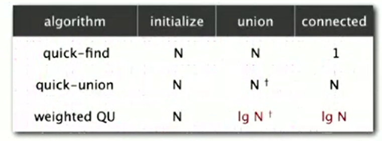
- Quick Find
- It's an eager algorithm to solve the dynamic connectivity problem
- Data structure description
- The data structure is an integer array
id[]of size N, each entry is the id that represents the connected component to which this point belongs - Connected command: if two points have the same id, then they are connected
- Union command: when union point
pto pointq, change all elements whose id equals toid[p]toid[q]
- The data structure is an integer array
- Algorithm
1
2
3
4
5
6
7
8
9
10
11
12
13
14
15
16
17
18
19
20
21
22
23
24
public class QuickFindUF {
private int[] id;
public QuickFindUF(int N) {
id = new int[N];
for (int i = 0; i < N; i++) {
id[i] = i;
}
}
public boolean connected(int p, int q) {
return id[p] == id[q];
}
public void union(int p, int q) {
int idp = id[p];
int idq = id[q];
for (int i = 0; i < N; i++) {
if (id[i] == idp) {
id[i] = idq;
}
}
}
} - Performance analysis: N union objects on N objects takes quadratic time, which is quite unbearable fo large datasets
- Quick Union
- It's a lazy approach to solve the dynamic connectivity problem
- Data structure description
- The data structure is an integer array
id[]of size N, each entry is the id that represents the parent point of the current point. All points construct a forest containing connected trees and unconnected leaves - Root of the tree containing point
iisid[id[id[...id[i]...]]] - Connected command: if two points have the same root, then they are connected
- Union command: when union point
pto pointq, set the parent of p's root be q's root
- The data structure is an integer array
- Algorithm
1
2
3
4
5
6
7
8
9
10
11
12
13
14
15
16
17
18
19
20
21
22
23
24
25
26
public class QuickUnionUF {
private int[] id;
public QuickUnionUF(int N) {
for (int i = 0; i < N; i++) {
id[i] = i;
}
}
private int root(int node) {
while(node != id[node]) {
node = id[node];
}
return node;
}
public boolean connected(int p, int q) {
return root(p) == root(q);
}
public void union(int p, int q) {
int rootp = root(p);
int rootq = root(q);
id[rootp] = rootq;
}
} - Performance analysis: trees can be too tall, then find command can be slow since it's a linear operation
- Quick Union Improvement
- Improvement 1: Weighting
- Keep track of size of each tree, and balance by linking root of smaller tree to root of larger tree in union command. When there are equal size trees, put the former tree under the latter tree
- Data structure description: same as quick union, but maintain extra
array
size[i]to count number of objects in the tree rooted ati - Find command: identical to quick union
- Union link root of smaller tree to root of larger tree, update the
size[] array
1
2
3
4
5
6
7
8
9
10
11
public void union(int p, int q) {
int rootp = root(p);
int rootq = root(q);
if (size(rootp) <= size(rootq)) {
id[rootp] = rootq;
size[rootq] += size[rootp];
} else {
id[rootq] = rootp;
size[rootp] += size[rootq];
}
} - Theorem: depth of any node x is at most lgN
- Performance analysis
- Improvement 2: Path Compression
- Idea: after computing the root of p, set the id of each examined
node to point to that root, so that the tree is flattened
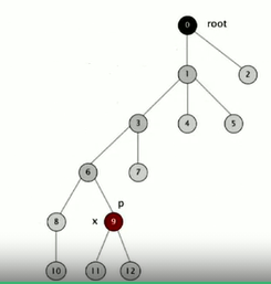 Convert the above tree
into the following one
Convert the above tree
into the following one 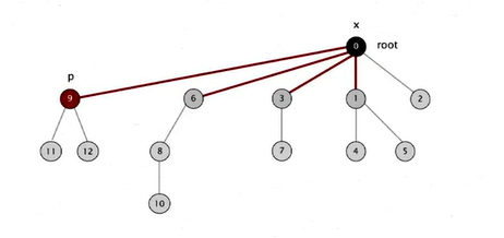
- Java implementation
- Two-pass implementation: add a second loop to
root()to set theid[]of each examined node to the root - Simpler one-pass variant: make every other node in path point to its
grandparent
1
2
3
4
5
6
7
private int root(int node) {
while (node != id[node]) {
id[node] = id[id[node]];
node = id[node];
}
return node;
}
- Two-pass implementation: add a second loop to
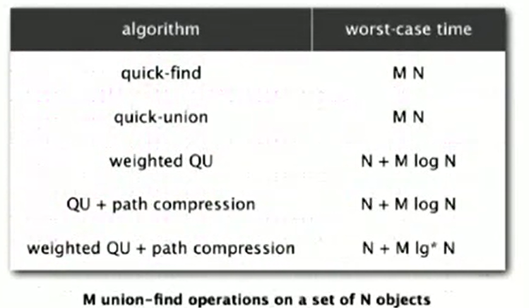
- Theorem: starting from an empty data structure, any sequence of M union-find operations on N objects makes \(\leq c(N + M lgN)\) array accesses. Actually there is no linear algorithm for the union find problem
- Idea: after computing the root of p, set the id of each examined
node to point to that root, so that the tree is flattened
- Summary
- Improvement 1: Weighting
- Union Find Application
- There are many applications for the union find problem
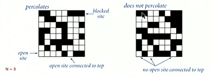
- Percolation
- It's a model for many physical systems
- There is N-by-N grid of sites, each site is open with probability
\(p\) or blocked with probability \(1 - p\). The system percolates iff the top
and bottom are connected by open sites
- Likelihood of percolation
When N is large, theory guarantees a sharp threshold \(p^{*}\)
If \(p \ge p^{*}\): almost certainly percolates
If \(p \le p^{*}\): almost certainly does not percolate
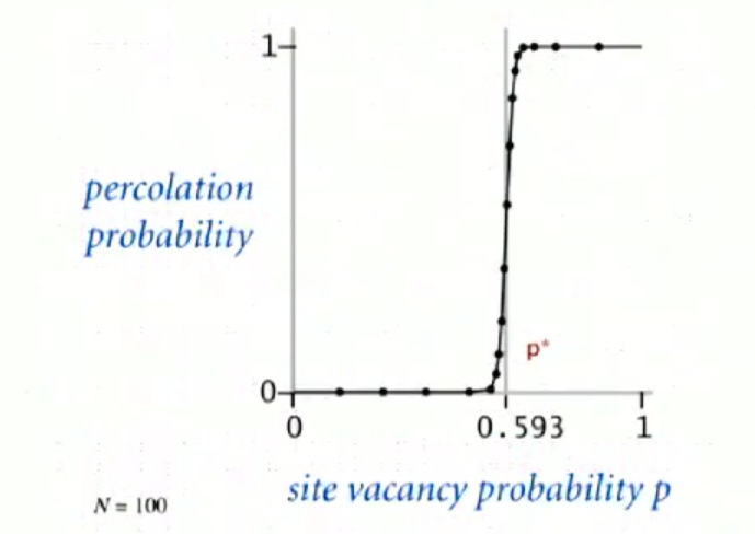
No analytical solution of \(p^{*}\) could be found, but it could be estimated using Monte Carlo simulation
- Initialize N-by-N whole grid to be blocked
- Declare random sites open until top connected to bottom
- Vacancy percentage estimates \(p^{*}\)
We can use dynamic connectivity to estimate the percolation threshold. For \(N = 100\), the estimated \(p^{*} \approx 0.592746\)
- Dynamic Connectivity
Week 2
- Stacks and Queues
- Fundamental data types:
- Value: collection of objects
- Operations: insert, remove, iterate, test if empty
- Stack: LIFO, insert is called push, remove is called pop
- Queue: FIFO, insert is called enqueue, remove is called dequeue
- Module programming: completely separate interface and implementation
- Stack
- Stack API
1
2
3
4
5
6
7
public class StackOfStrings {
StackOfStrings()
void push(String item)
String pop()
boolean isEmpty()
int size()
} - LinkedList Implementation
1
2
3
4
5
6
7
8
9
10
11
12
13
14
15
16
17
18
19
20
21
22
23
24
25
public class LinkedListStack {
private Node first = null;
private class Node {
String item;
Node next;
}
public String pop() {
String item = first.item;
first = first.next;
return item;
}
public void push(String item) {
Node oldFirst = first;
first = new Node();
first.item = item;
first.next = oldFirst;
}
public boolean isEmpty() {
return first == null;
}
}- Every operation takes constant time in the worst case
- Array Implementation
1
2
3
4
5
6
7
8
9
10
11
12
13
14
15
16
17
18
19
20
21
22
23
24
25
26
27
public class ArrayStack {
private String[] items;
private int N = 0;
public ArrayStack(int capacity) {
items = new String[capacity];
}
public boolean isEmpty() {
return N ==0;
}
public void push(String item) {
items[N++] = item;
}
/* Loitering
public String pop() {
return items[--N];
}
*/
public String pop() {
String item = items[--N];
items[N] = null;
return item;
}
}- Don't address underflow(pop with an empty stack) and overflow(push with a full stack)
- Loitering: holding a reference to an object when it is no longer needed
- Stack API
- Resizing Arrays
First try: change size by 1 for push and pop
- It's too expensive, you need to copy all items to the new array. In order to insert \(N\) items into an empty stack, it costs \(N^2\) time(To insert into a full stack with \(k\) size, you need to create a \(k + 1\) array and copy all items, so that's \(1 + ... + N \sim N^2\))
Repeated doubling: double array size when full, halve array size when one-quarterfull
1
2
3
4
5
6
7
8
9
10
11
12
13
14
15
16
17
18
19
20
21
22
23
24
25
26
27
28
public class ArrayStack {
private String[] items = new String[1];
private N = 0;
public void push(String item) {
if (N == items.length) {
resize(2 * items.length);
}
items[N++] = item;
}
public String pop() {
String item = items[--N];
items[N] = null;
if (N > 0 && N == items.length /4) {
resize(items.length / 2)
}
return item;
}
private void resize(int capacity) {
String[] copy = new String[capacity];
for (int i = 0; i < N; i++) {
copy[i] = items[i];
}
items = copy;
}
}- To insert N items into an empty array, it costs \(N + 2 + 4 + ... + N \sim 3N\)
- Amortized analysis: average running time per operation over a worst-case sequence of operations
- Starting from an empty stack, any sequence of \(M\) push and pop operations takes time proportional to \(M\)
- LinkedList v.s. resizing array for stack implementation
- LinkedList: every operation takes constant time in the worst case, use extra time and space to deal with the links
- Resizing-array: every operation takes constant amortized time, less wasted space
- Queues
- Queue API
1
2
3
4
5
6
7
public class QueueOfStrings {
QueueOfStrings()
void enqueue(String item)
String dequeue()
boolean isEmpty()
int size()
} - LinkedList Implementation
1
2
3
4
5
6
7
8
9
10
11
12
13
14
15
16
17
18
19
20
21
22
23
24
25
26
27
28
29
30
31
32
33
public class LinkedListQueue {
private Node first;
private Node last;
private class Node {
String item;
Node next;
}
public String dequeue() {
String item = first.item;
first = first.next;
if (isEmpty()) {
last = null;
}
return item;
}
public void enqueue(String item) {
Node oldLast = last;
last = new Node();
last.item = item;
last.next = null;
if (isEmpty()) {
first = last;
} else {
oldLast.next = last;
}
public boolean isEmpty() {
return first == null;
}
} - Resizing Array Implementation
1
2
3
4
5
6
7
8
9
10
11
12
13
14
15
16
17
18
19
20
21
22
23
24
25
26
27
28
29
30
public class ArrayQueue {
private String[] items = new String[1];
private int front = 0;
private int rear = 0;
public void enqueue(String item) {
if (rear - front == items.length) {
resize(2 * items.length);
}
items[rear] = item;
rear += 1;
}
public String dequeue() {
String item = items[front];
items[front] = null;
front += 1;
if ( rear - front > 0 && rear - front == items.length / 4) {
resize(items.length / 2);
}
}
public void resize(int capacity) {
String[] copy = new String[capacity];
for (int i = 0; i < rear - front; i++) {
copy[i] = items[front + i];
}
items = copy;
}
}
- Queue API
- Generics
- Collections that can contain various types data
- Implement a separate collection class for each type: tedious
- Implement a collection for object type and use type casting like: Object variable = new Object(); T target = (T) variable
- Implement a collection with generics: avoid casting when using collections, discover type mismatch errors at compile-time rather than run-time
- LinkedList Stack with Generics
1
2
3
4
5
6
7
8
9
10
11
12
13
14
15
16
17
18
19
20
21
22
23
24
public class LinkedListStackGeneric<T> {
private Node first = null;
private class Node {
T item;
Node next;
}
public void push(T item) {
Node oldFirst = first;
first = new Node();
first.item = item;
first.next = oldFirst;
}
public T pop() {
T item = first.item;
first = first.next;
return item;
}
public boolean isEmpty() {
return first == null;
}
} - ArrayStack with Generics
1
2
3
4
5
6
7
8
9
10
11
12
13
14
15
16
17
18
19
20
21
22
23
public class ArrayStackGeneric<T> {
private T[] items;
private int N = 0;
public ArrayStackGeneric(int capacity) {
// It's not allowed in java to create generic arrays, you need type casting here
s = (T[]) new Object[capacity];
}
public boolean isEmpty() {
return N ==0;
}
public void push(T item) {
items[N++] = item;
}
public T pop() {
T item = items[--N];
items[N] = null;
return item;
}
}- Autoboxing
- For each primitive type there is a wrapper object type, automatic cast ca be done between primitive type and wrapper type
- You need to use wrapper types rather than primitive types in collections
- Convert from String to other type:
int aInt = Integer.parseInt("aString");
- Autoboxing
- Collections that can contain various types data
- Iterators
- Java supports iteration over stack items by client, without revealing the internal representation of the collections
- Iterable: a interface that has a method that returns an Iterator
1
2
3
public interface Iterable<Item> {
Iterator<Item> iterator();
} - Iterator: an interface that has methods
hasNext()andnext()1
2
3
4public interface Iterator<Item> {
boolean hasNext();
Item next();
} - Java supports elegant enhanced-for loop with iterable data
structures
1
2
3for(String element: stack) {
System.out.println(element);
} - LinkedList Stack with Iterator
1
2
3
4
5
6
7
8
9
10
11
12
13
14
15
16
17
18
19
20
21
public class LinkedListStack<T> implements Iterable<T> {
...
public Iterator<T> iterator() {
return new ListIterator();
}
private class ListIterator implements java.util.Iterator<T> {
private Node current = first;
public boolean hasNext() {
return current != null;
}
public T next() {
T item = current.item;
current = current.next;
return item;
}
}
} - Array List Stack with Iterator
1
2
3
4
5
6
7
8
9
10
11
12
13
14
15
16
17public class ArrayStack<T> implements Iterable<T> {
public Iterator<T> iterator() {
return new ArrayIterator();
}
private class ArrayIterator implements Iterator<T> {
private int i = N;
public boolean hasNext() {
return i > 0;
}
public T next() {
return items[--i];
}
}
} - Bag
- Application: adding items to a collection and iterating, order doesn't matter
- Bag API
1
2
3
4
5
6public class Bag<T> implements Iterable<T> {
Bag();
void add(T item);
int size();
Iterable<T> iterator();
}
- Stack and Queue Applications
- Java collections library
- List
- List interface:
java.util.List: public interface List<E> extends Collection<E> - Implementations:
java.util.ArrayList: public class LinkedList<E> extends AbstractSequentialList<E> implements List<E>, Deque<E>, Cloneable, java.io.Serializable,java.util.LinkedList: public class LinkedList<E> extends AbstractSequentialList<E> implements List<E>, Deque<E>, Cloneable, java.io.Serializable
- List interface:
- Stack:
java.util.Stack: public class Stack<E> extends Vector<E> - Queue:
java.util.Queue: public interface Queue<E> extends Collection<E>
- List
- Stack applications:
- Parsing in a complier
- Dijkstra's two-stack algorithm
- Operand: push into the operand stack
- Operator: push into the operator stack
- Left parenthesis: ignore
- Right parenthesis: pop operator and two operands, calculate, push the result into the operand stack
- Dijkstra's two-stack algorithm
- Java virtual machine
- Undo in a word processor
- Back button in a web browser
- ...
- Parsing in a complier
- Java collections library
- Problems
- Create a queue using two stack
1
2
3
4
5
6
7
8
9
10
11
12
13
14
15
16
17
18
19
20
21
22
23
24
25
26
27
28
29
30
31
32
33
34
35
36
37
38
39
40
41
42
43
44
45
46
47
48
49
50
51
52
53
54
55
56
57
58
59
60
61
62
63
64
65
66
67
68
69
70
71// You should not use java.util.Stack, you should use java.util.Deque instead:
// A more complete and consistent set of LIFO stack operations is provided by the
// Deque interface and its implementations, which should be used in preference to this class.
//Space complexity: O(N), time complexity: O(N)
class MyQueue {
Deque<Integer> out, in;
public MyQueue() {
in = new ArrayDeque<>();
out = new ArrayDeque<>();
}
public void push(int x) {
while (!out.isEmpty()) {
in.addLast(out.pollLast());
}
in.addLast(x);
}
public int pop() {
while (!in.isEmpty()) {
out.addLast(in.pollLast());
}
return out.pollLast();
}
public int peek() {
while (!in.isEmpty()) {
out.addLast(in.pollLast());
}
return out.peekLast();
}
public boolean empty() {
return out.isEmpty() && in.isEmpty();
}
}
//Time complexity: amortized O(1), space complexity: O(N)
class MyQueue {
Deque<Integer> out, in;
public MyQueue() {
in = new ArrayDeque<>();
out = new ArrayDeque<>();
}
public void push(int x) {
in.addLast(x);
}
public int pop() {
if (out.isEmpty()) {
while (!in.isEmpty()) {
out.addLast(in.pollLast());
}
}
return out.pollLast();
}
public int peek() {
if (out.isEmpty()) {
while (!in.isEmpty()) {
out.addLast(in.pollLast());
}
}
return out.peekLast();
}
public boolean empty() {
return out.isEmpty() && in.isEmpty();
}
} - Max/Min Stack: use another stack to trace the max/min value
- Create a queue using two stack
- Fundamental data types:
- Elementary Sorts
- Sorting Introduction
- Callbacks
- Goal: sort any type of data
- Client passes array of objects to
sort()function, the sort function calls back object'scompareTo()method as needed
- Implementing callbacks
- Java: interface
1
2
3
4
5public interface Comparable<Item> {
public int compareTo(Item that);
}
// v.compareTo(w) returns negative integer, zero, or positive if v < w, v == w, or v > w
// if v and w are not comparable, throws an Exception - C: function pointers
- C++: class-type pointers
- Python, Perl, Javascript: first-class functions
- Java: interface
- Total order:
- Antisymmetry: if \(v \leq w\) and \(w \leq v\), then \(v = w\)
- Transitivity: if \(v \leq w\) and \(w \leq x\), then \(v \leq x\)
- Totality: either \(v \leq w\) or \(w \leq v\) or both
- Callbacks
- Selection Sort
- Idea to get an ascending array
- In iteration i, find index
minof smallest remaining entry - Swap
array[i]andarray[min] - The part on the left side of i is an invariant, that is, the entries are sorted
- In iteration i, find index
- Implementation
1
2
3
4
5
6
7
8
9
10
11
12
13
14
15
16public class SelectionSort {
public static void sort(Comparable[] items) {
int N = items.length;
for (int i = 0; i < N; i++) {
int min = i;
for (int j = i + 1; j < N; j++) {
if (items[j].compareTo(items[min]) < 0) {
min = j;
}
}
Comparable item = items[min];
items[min] = items[i];
items[i] = item;
}
}
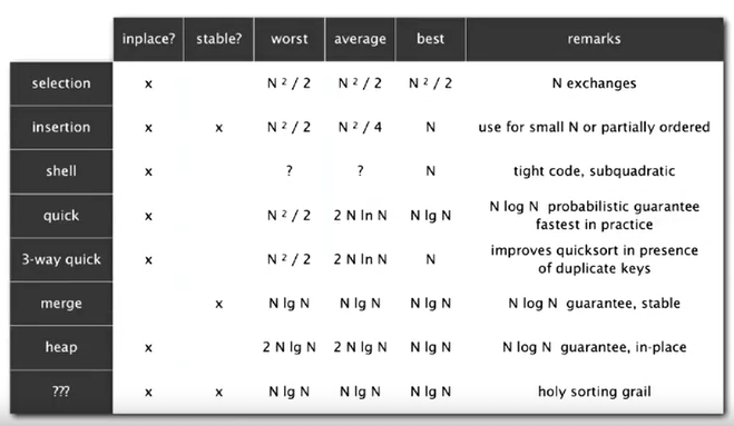
} - For an array with size \(N\), selection sort takes about \(\frac{N^2}{2}\) comparisons and about \(N\) exchanges. No matter whether the input is sorted or totally unsorted, the complexity of selection sort is always quadratic
- Idea to get an ascending array
- Insertion Sort
- Idea to get an ascending array
- In iteration i, swap
array[i]with each larger entry to its left - The part on the left side of i is an invariant, that is, the entries are sorted
- In iteration i, swap
- Implementation
1
2
3
4
5
6
7
8
9
10
11
12public class InsertionSort {
public static void sort(Comparable[] items) {
int N = items.length;
for (int i = 0; i < N; i++) {
for (int j = i; j > 0 && items[j].compareTo(items[j - 1]) < 0; j--) {
Comparable item = items[j];
items[j] = items[i];
items[i] = item;
}
}
}
} - For a randomly-ordered array with \(N\) distinct keys, insertion sort uses about \(\frac{N^2}{4}\) comparisons and about \(\frac{N^2}{4}\) exchanges on average.
- For an ordered array, insertion sort makes \(N - 1\) comparisons and \(0\) exchanges
- For an reversely-ordered array, insertion sort makes about \(\frac{N^2}{2}\) comparisons and about \(\frac{N^2}{4}\) exchanges
- Idea to get an ascending array
- Shell Sort
- Idea to get an ascending array
- Move entries more than one position at a time by h-sorting the array
- Use insertion sort in h-sorting: for large h, the subarray is small, so sorting can be fast, for small h, the array is nearly sorted, to insertion sort is fast
- A m-sorted array is still m-sorted after being n-sorted
- The general chosen h is \(h = 3 * h + 1\)
- Implementation
1
2
3
4
5
6
7
8
9
10
11
12
13
14
15
16
17
18
19public class ShellSort {
public static void sort(Comparable[] items) {
int N = items.length;
int h = 1;
while (h < N /3) {
h = 3 * h + 1;
}
while (h >= 1) {
for (int i = h; i < N; i++) {
for (int j = i; j >= h && items[j].compareTo(items[j - h]) < 0; j -= h) {
Comparable item = items[j];
items[j] = items[j - h];
items[j - h] = item;
}
h = h / 3;
}
}
}
} - The worst-case number of comparisons used by shell sort with \(3 * h + 1\) increments is \(O(N^{\frac{3}{2}})\)
- Shell sort is faster than selection sort and insertion sort, the larger the array is, the better the performance is
- Idea to get an ascending array
- Shuffling Sort
- Initial idea to get a randomized shuffle of an array
- Generate a random real number for each array entry
- Sort the array
- Shuffle sort produces a uniformly random permutation of the input array, provided no duplicate values
- Knuth shuffle in linear time
- In iteration i, pick integer r between 0 and i uniformly at random
- Swap
array[r]andarray[i] - The part on the left side of i is an invariant, that is, the entries are uniformly randomized
- Implementation
1
2
3
4
5
6
7
8
9
10
11public class ShuffleSort {
public static void sort(Comparable[] items) {
int N = items.length;
for (int i = 0; i < N; i++) {
int r = StdRandom.uniform(i + 1); // Uniform random number in [0, i]
Comparable item = items[r];
items[r] = items[i];
items[i] = item;
}
}
}
- Initial idea to get a randomized shuffle of an array
- Convex Hull
- Some equivalent definitions of a convex hull
- The smallest perimeter fence enclosing a set of points
- The smallest convex set containing all the points
- The smallest area convex polygon enclosing the points
- The convex polygon enclosing the points, whose vertices are points in set
- Output: sequence of vertices in counterclockwise order
- Fact
- Can traverse the convex hull by making only counterclockwise turns
- The vertices of convex hull appear in increasing order of polar angle with respect to point p with lowest y-coordinate
- Graham Scan
- Choose point p with smallest y-coordinate
- Sort points by polar angle with p
- Consider points in order, discard unless it creates a counterclockwise turn
- Some equivalent definitions of a convex hull
- Sorting Introduction
Week 3
- Merge Sort
- Introduction
- Two classic sorting algorithm
- Merge sort: java sort for objects, Perl, C stable sort, Python stable sort, Firefox javascript, ...
- Quick sort: java sort for primitive types, C qsort, Unix, C++, Python, Matlab, Chrome javascript, ...
- Idea is divide and conquer
- Divide the array into two halves
- Recursively sort each half
- Merge the two halves using an auxiliary array
- Implementation
1
2
3
4
5
6
7
8
9
10
11
12
13
14
15
16
17
18
19
20
21
22
23
24
25
26
27
28
29
30
31
32
33
34
35
36
37
38
39
40
41
42public class MergeSort {
private static Comparable[] aux;
public static void sort(Comparable[] items) {
aux = new Comparable[a.length]; // Do not create aux in the private recursive sorts
sort(items, 0, items.length - 1);
}
private static void sort(Comparable[] items, int lo, int hi) {
if (hi <= lo) {
return;
}
int mid = lo + (hi - lo) / 2;
sort(items, lo, mid);
sort(items, mid + 1, hi);
merge(items, lo, mid, hi);
}
private static void merge(Comparable[] items, int lo, int mid, int hi) {
// assert isSorted(items, lo, mid);
// assert isSorted(items, mid + 1, hi);
for (int i = 0; i <= hi; i++) {
aux[i] = items[i];
}
int i = lo; j = mid + 1;
for(int k = lo; k <= hi; k++) {
if (i > mid) {
items[k] = aux[j++]; // items[lo...mid] has already been copied
} else if (j > hi) {
items[k] = items[i++]; // items[mid + 1...hi] has already been copied
} else if (aux[j].compareTo(aux[i]) < 0) {
items[k] = aux[j++]; // For stability reason, we cannot revert this else if statement and the else statement
} else {
items[k] = aux[i++];
}
}
// assert isSorted(items, lo, hi)
}
} - Facts
- Merge sort uses at most \(NlogN\) comparisons and \(6NlogN\) array access to sort any array of size \(N\). If \(D(N)\) satisfies \(D(N) = 2D(\frac{N}{2}) + N\) for \(N > 1\), with \(D(1) = 0\), then \(D(N) = N logN\)
- Merge sort uses extra space proportional to \(N\)
- A sorting algorithm is in-place if it uses \(\leq clogN\) extra memory. Ex. insertion sort, selection sort, shell sort. Merge sort can be in-place, [Kronrod, 1969]
- Improvements
- Merge sort is recursive, so it will be slow for small subarrays, we
can use insertion sort for small subarrays
1
2
3
4
5
6
7
8
9
10
11
12private int FUTOFF = 7; // you can set your own cutoff to decide how small is an small array
private static void sort(Comparable[] items, int lo, int hi) {
if (hi <= lo + CUTOFF - 1) {
InsertionSort.sort(items, lo, hi);
return;
}
int mid = lo + (hi - lo) / 2;
sort(items, aux, lo, mid);
sort(items, aux, mid + 1, hi);
merge(items, aux, lo, mid, hi);
} - If
items[mid] <= items[mid + 1], then don't need to merge, the whole array is already sorted1
2
3
4
5
6
7
8
9
10
11
12
13
14private static void sort(Comparable[] items, int lo, int hi) {
if (hi <= lo + CUTOFF - 1) {
InsertionSort.sort(items, lo, hi);
return;
}
int mid = lo + (hi - lo) / 2;
sort(items, aux, lo, mid);
sort(items, aux, mid + 1, hi);
if (items[mid].compareTo(items[mid + 1]) < 0) {
return;
}
merge(items, aut, lo, mid, hi);
} - Eliminate the copy to the auxiliary array
1
2
3
4
5
6
7
8
9
10
11
12
13
14
15
16
17
18
19
20
21
22
23
24
25
26
27
28
29
30
31private static void merge(Comparable[] items, Comparable[] aux, int lo, int mid, int hi) {
int i = lo;
int j = mid + 1;
for(int k = lo; k <= hi; k++) {
if (i > mid) {+
aux[k] = items[j++]
} else if (j > hi) {
aux[k] = items[i++]
} else if (items[j].compareTo(items[i]) < 0) {
aux[k] = items[j++]
} else {
aux[k] = items[i++];
}
}
}
private static void sort(Comparable[] items, Comparable[] aux, int lo, int hi) {
if (hi <= lo + CUTOFF - 1) {
InsertionSort.sort(items, lo, hi);
return;
}
int mid = lo + (high - lo) / 2;
sort(aux, items, lo, mid);
sort(aux, items, mid + 1, hi);
if (aux[mid].compareTo(aux[mid + 1]) < 0) {
return;
}
merge(aux, items, lo, mid, hi);
}
- Merge sort is recursive, so it will be slow for small subarrays, we
can use insertion sort for small subarrays
- Two classic sorting algorithm
- Bottom-up Merge Sort
- No recursion needed plan
- Pass through array, merging subarrays of size 1
- Repeat for subarrays of size 2, 4, 6, 8, 16, ..., array.length
- Implementation
1
2
3
4
5
6
7
8
9
10
11
12
13
14
15
16
17
18
19
20
21
22
23
24
25
26
27
28
29
30public class MergeSort {
private static Comparable[] aux;
private static void merge(Comparable[] items, int lo, int mid, int hi) {
int i = lo;
int j = mid + 1;
for (int k = lo; k <= hi; k++) {
if (i > mid) {
items[k] = aux[j++];
} else if (j > hi) {
items[k] = aux[i++];
} else if (aux[j].compareTo(aux[i]) < 0) {
items[k] = aux[j++];
} else {
items[k] = aux[i++];
}
}
}
public static void sort(Comparable[] a) {
int N = items.length;
aux = new Comparable[N];
for(int sz = 1; sz < N; sz *= 2) {
for(int lo = 0; lo < N - sz; lo += sz * 2) {
merge(items, lo, lo + sz - 1, Math.min(lo + sz * 2 - 1, N -1));
}
}
}
}
- No recursion needed plan
- Sorting Complexity
- Complexity of sorting
- Computational complexity: framework to study efficiency of algorithms for solving a particular problem X
- Model of computation: allowable operations
- Cost model: operation counts
- Upper bound: cost guarantee provided by some algorithm for X
- Lower bound: proven limit on cost guarantee of all algorithms for X
- Optimal algorithm: algorithm with best possible cost guarantee for X
- Sorting Ex.
- Model of computation: decision tree
- The height of the tree is the worst-case number of comparisons
- There is at least one leaf for each possible ordering
- Cost model: number of comparisons
- Upper bound: about \(NlogN\) from merge sort
- Lower bound: Any compare-based sorting algorithm must at least \(lg(N!) \sim NlgN (Stirling's formula)\) comparisons in the worst-case
- Optimal algorithm:merge sort is an optimal algorithm
- Model of computation: decision tree
- Merge sort is optimal with respect to number of comparisons but it's not optimal with respect to space usage
- Complexity results in context: if more information is provided in
terms of the initial order of input, the distribution of key values, or
the representation of the keys, lower bound may not hold
- Partially-ordered array: insertion sort requires only \(N - 1\) comparisons if input is sorted
- Duplicate keys: three-way quick sort can be used
- Digital properties of keys: use digit/character comparisons instead of key comparisons for number and strings, radix sort is used here
- Complexity of sorting
- Comparators
Comparable interface: sort using a type's natural order
Comparator interface: sort using an alternate order, the order must be a total order
1
2
3
4
5
6public interface Comparator <Key> {
int compare(Key v, Key w);
// If v is less than w, then compare(v, w) < 0ssss
// If v equals to w, then compare(v, w) == 0
// If v is larger than w, then compare(v, w) > 0
}Usage in
Arrays.sort()- Create Comparator instance, the instance is an object of a class that implements the Comparator interface
- Pass as second argument to
Arrays.sort()
- Stability
- A stable sort preserves the relative order of items with equal keys.
If in the original array we have
array[i] == array[j], and i < j, then in the sorted array,array[i]should still appear ahead ofarray[j] - Insertion sort and merge sort are stable, selection sort and shell
sort are not stable. You need to check how the
compareTo()method or thecompare()method is implemented
- Insertion sort: we check
j > 0 && items[j].compareTo(items[j - 1]) < 0, so no equal items never move past each other - Selection sort: there may be a long-distance exchange that might
move an item past some equal item, here we
swap(array[i], array[min]), where min is in {i + 1, ..., array.length - 1} - Merge sort: it's stable as long as merge operation is stable, and in
the merge function, we have hence if there is an equal situations(
1
2
3
4
5else if (aux[j].compareTo(aux[i]) < 0) {
items[k] = aux[j++];
} else {
items[k] = aux[i++];
}aux[j] == aux[i]), we use the left partaux[i]so that we will not change the relative order ofaux[i]andaux[j], therefore it's stable - Shell sort: there is a long-distance exchange in shell sort so it's
not stable, we
swap(array[j], array[j - h]), there may be values that are equal toarray[j - h]in the interval of[j - h + 1, , j - 1], so it's not stable - Question:
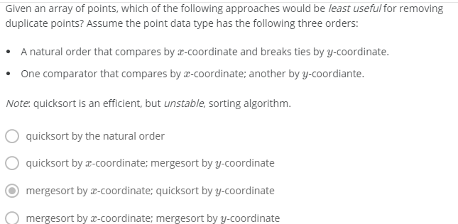
- We only need to care about situation where \(x_0 = x_1, and \; y_0 = y_1\), if these points can be put near each other, then it's fine
- Choice A: A is fine
- Choice B: quick sort x, so x is in order, merge sort y will not change the sorted x since it's stable
- Choice C: merge sort x, so x is in order, quick sort y may change the sorted x since it's unstable
- Choice D: merge sort is stable
- A stable sort preserves the relative order of items with equal keys.
If in the original array we have
- Problems:
- Suppose that the subarray
a[0]toa[n - 1]is sorted, and the subarraya[n]toa[2 * n - 1]is sorted. How can you merge the two subarrays so that array a is sorted using an auxiliary array of length n instead of 2n?1
2
3
4
5
6
7
8
9
10
11
12
13
14
15
16
17
18
19public void mergeWithShortAux(Comparable[] a, Comparable[] aux) {
int N = a.length / 2;
for (int i = 0; i < N; i++) {
aux[i] = a[i];
}
int i = 0;
int j = N;
for (int k = 0; i < a.length; k++) {
if (i > N) {
a[k++] = a[j++];
} else if (j > a.length) {
a[k++] = a[i++];
} else if(a[j].CompareTo(aux[i]) < 0) {
a[k++] = a[j++];
} else {
a[k++] = aux[i++];
}
}
} - An inversion in an array
a[]is a pair of entriesa[i]anda[j]such thati < jbuta[i] > a[j]. Given an array, design a linearithmic algorithm to count the number of inversions.1
2
3
4
5
6
7
8
9
10
11
12
13
14
15
16
17
18
19
20
21
22
23
24
25
26
27
28
29
30
31
32
33
34
35
36
37
38//Obviously there is an O(n^2) solution, for i in range(len(a)), if a[j] > a[i] for j in range(i + 1, len(a)), then count ++
// The following one is from https://www.youtube.com/watch?v=Vj5IOD7A6f8
//Idea inversion in a = recursive count (left half) + recursive count (right half) + merge count(left + right)
private int merge(Comparable[] a, Comparable[] aux, int lo, int mid, int hi) {
for (int k = lo; k <= hi; k++) {
aux[k] = a[k];
}
int i = lo, j = mid + 1, count = 0;
for (int k = lo; k <= hi; k++) {
if (i > mid)
a[k] = aux[j++];
else if (j > hi)
a[k] = aux[i++];
else if (aux[i].compareTo(aux[j]) > 0) {
a[k] = aux[j++];
count += mid - i + 1;
} else {
a[k] = aux[i++];
}
}
return count;
}
private int sort(Comparable[] a, Comparable[] aux, int lo, int hi) {
if (lo >= hi) return 0;
int mid = lo + (hi - lo)/2;
int count1 = sort(a, aux, lo, mid);
int count2 = sort(a, aux, mid + 1, hi);
int count3 = merge(a, aux, lo, mid, hi);
return count1 + count2 + count3;
}
public int inverseionCount(Comparable[] a) {
Comparable[] aux = new Comparable[a.length];
return sort(a, aux, 0, a.length - 1);
}
- Suppose that the subarray
- Introduction
- Quick Sort
- Introduction
- Ieda
- Randomly shuffle the array
- Partition the array, so that for some j,
array[i]is in place, no larger entry to the left of j, no smaller entry to the right of j - Sort each piece recursively
- Partition
- Phase I: repeat until i and j pointers cross
- Scan i from left to right so long as
array[i] < array[lo] - Scan j from right to left so long as
array[j] > array[lo] - Exchange
array[i]witharray[j]
- Scan i from left to right so long as
- Phase II: when pointers cross.
- Exchange
array[j]witharray[lo]
- Exchange
- Phase I: repeat until i and j pointers cross
- Java implementation
1
2
3
4
5
6
7
8
9
10
11
12
13
14
15
16
17
18
19
20
21
22
23
24
25
26
27
28
29
30
31
32
33
34
35
36
37
38
39
40public class QuickSort{
private static int partition(Comparable[] items, int lo, int hi) {
int i = lo, j = hi + 1;
while (true) {
while (items[++i].compareTo(items[lo]) < 0) {
if (i == hi) {
break;
}
}
while (items[--j].compareTo(items[lo]) > 0) {
if (j == lo) {
break;
}
}
if (i >= j) {
break;
}
}
Comparable item = items[j];
items[j] = items[lo];
items[lo] = item;
return j;
}
private static void sort(Comparable[] items, int lo, int hi) {
if (hi <= lo) {
return;
}
int j = partition(items, lo, hi);
sort(items, lo, j - 1);
sort(items, j + 1, hi);
}
public static void sort(Comparable[] items) {
StdRandom.shuffle(items);
sort(items, 0, items.length - 1);
}
} - Implementation Comments
- The partition in quick sort is in-place, compared with merge sort, quick sort does not take any extra space
- Testing whether the pointers cross is a bit trickier than it might seem, especially when there are duplicate keys
- Testing
j ==lois redundant, but testingi == hiis not - Random shuffling is needed for performance guarantee
- When duplicates are present, it is better to stop on keys equal to the partitioning item's key
- Performance analysis
- On average, quick sort makes \(\sim 2NlogN\) comparisons and \(\sim \frac{1}{3}NlogN\) exchanges
- In best cases, quick sort makes \(\sim NlogN\) comparisons
- In worst cases, quick sort makes \(\sim \frac{1}{2} N^{2}\) comparisons, randomly shuffling can avoid these situations
- Properties
- Quick sort is an in-place sorting algorithm
- Quick sort is not stable
- Ieda
- Selection
- Goal: given an array of \(N\) items, find the \(k^{th}\) largest
- Applications: order statistics, find the top k
- Quick-select
- Partition array so that:
- Entry
array[j]is in place - No larger entry to the left of j
- No larger entry to the right of j
- Entry
- Repeat in one subarray, depending on j; finished when
j == k
- Partition array so that:
- Java implementation
1
2
3
4
5
6
7
8
9
10
11
12
13
14
15
16public static Comparable select(Comparable[] items, int k) {
StdRandom.shuffle(items);
int lo = 0, hi = items.length - 1;
while (hi > lo) {
int j = partition(items, lo, hi);
if (j < k) {
lo = j + 1;
} else if (j > k) {
hi = j - 1;
} else {
return items[k]
}
}
return items[k];
} - Quick-select takes linear time on average
- Duplicate Keys
- Merge sort with duplicate keys: always between \(\frac{1}{2}NlogN\) and \(NlogN\) comparisons
- Quick sort with duplicate keys: algorithm goes quadratic unless partitioning stops on equal keys
- Dijkstra three-way partitioning quick sort
- Let v be partitioning item
items[lo] - Scan i from left to right:
- If
items[i] < v: exchangeitems[lt]withitems[i], increase both lt and i - If
items[i] > v: exchangeitems[gt]withitems[i], decrease gt - If
items[i] == v: increase i
- If
- Java implementation
1
2
3
4
5
6
7
8
9
10
11
12
13
14
15
16
17
18
19
20
21
22
23
24
25
26
27
28public class Quick3Way {
private static void sort(Comparable[] items, int lo, int hi) {
if (hi <= lo) {
return;
}
int lt = lo, i = lo + 1, gt = hi;
Comparable v = items[lo];
while (i <= gt) {
int cmpt = items[i].compareTo(v);
if (cmp < 0) {
Comparable item = items[i];
items[i] = items[lt];
items[lt] = item;
lt++;
i++;
} else if (cmp > 0) {
Comparable item = items[i];
items[i] = items[gt];
items[gt] = item;
gt--;
} else {
i++;
}
}
sort(items, lo, lt - 1);
sort(items, gt + 1, hi);
}
} - Quick sort with 3-way partitioning is entropy-optimal
- Randomized quick sort with 3-way partitioning reduces running time from linearithmic to linear in board class of applications
- Let v be partitioning item
- System Sorts
Arrays.sort()- Uses tuned quick sort for primitive types; uses tuned merge sort for
objects. For objects, merge sort is stable and guarantees \(NlogN\) performance, for primitive types,
quick sort uses less memory and is faster in generals. If you
deliberately create primitive inputs without proper shuffling, the
Arrays.sort()with quick sort can fail. - Has different method for each primitive type
- Has a method for data types that implements Comparable
- Has a method that uses a Comparator
- Uses tuned quick sort for primitive types; uses tuned merge sort for
objects. For objects, merge sort is stable and guarantees \(NlogN\) performance, for primitive types,
quick sort uses less memory and is faster in generals. If you
deliberately create primitive inputs without proper shuffling, the
- Which sort to choose
- Internal sort:
- Insertion sort, selection sort, bubble sort, shaker sort
- Quick sort, merge sort, heap sort, sample sort, shell sort
- Solitaire sort, red-black sort, splay sort, Yaroslavskiy sort, psort
- External sort: Poly-phase merge sort, cascade-merge, oscillating sort
- String/radix sorts: distribution, MSD, LSD, 3-way string quick sort
- Parallel sort:
- Bitonic sort, Batcher even-odd sort
- Smooth sort, cube sort, column sort
- GPU sort
- Internal sort:
- Application attributes to consider: stable, parallel, deterministic, keys all distinct, multiple key types, linked list or arrays, large or small items, large or small items, is your array randomly ordered, need guarantee performance
- Sort summary

- Problems
- Selection in two sorted arrays. Given two sorted arrays
a[]andb[], of length \(n_1\) and \(n_2\) and an integer \(0 \leq k \leq n_1 + n_2\), design an algorithm to find a key of rank k.- Solution 1: merge
a[]andb[]intoc[]where c[] is ordered with length \(n_1 + n_2\), pick c[k - 1] - Solution 2: compare
a[i]andb[j], usecountto track number of comparisons, ifcount == k, returna[count]orb[count]
- Solution 1: merge
- Selection in two sorted arrays. Given two sorted arrays
- Introduction
Week 4
- Priority Queues
- API and Elementary Implementations
API
1
2
3
4
5
6
7
8
9public class MaxPQ<Key extends Comparable<Key>> {
MaxPQ(); // create an empty priority queue
MaxPQ(Key[] items); // create a priority queue with given keys
void insert(Key v); // insert a key into the priority queue
Key delMax(); // return and remove the largest key
boolean isEmpty(); // is the priority queue empty
Key max(); // return the largest key
int size(); // number of entries in the priority queue
}Applications
- Event-driven simulation: customers in a line
- Data compression: huffman codes
- Graph searching: Dijkstra's algorithm, Prim's algorithm
- AI: A* search
- Operating systems: load balancing, interrupt handling
- Spam filtering: Bayesian spam filter
Unordered Array Implementation
1
2
3
4
5
6
7
8
9
10
11
12
13
14
15
16
17
18
19
20
21
22
23
24
25
26
27
28
29
30
31
32
33
34
35
36
37
38
39public class UnorderedMaxPQ<Key extends Comparable<Key>> {
private Key[] pq;
private int N;
public UnorderedMaxPQ(int capacity) {
pq = (Key[])new Comparable[capacity];
}
public boolean isEmpty() {
return N == 0;
}
public void insert(Key key) {
pq[N++] = key;
}
public Key delMax() {
int max = 0;
for (int i = 1; i < N; i++) {
if (pq[i].compareTo(pq[max]) > 0) {
max = i;
}
}
Key item = pq[max];
pq[max] = pq[N - 1];
pq[N - 1] = item;
return pq[--N];
}
public Key max() {
int max = 0;
for (int i = 1; i < N; i++) {
if (pq[i].compareTo(pq[max]) > 0) {
max = i;
}
}
return pq[max];
}
}Challenge: implement all operations efficiently
Implementation insert del max max unordered array 1 \(N\) \(N\) ordered array \(N\) 1 1 goal 1 1 1
- Binary Heaps
Binary tree: empty or node with links to left and right binary trees
Complete tree: perfectly balanced, except for bottom level
- Height of complete tree with \(N\) nodes is \(\left[ logN \right]\)
Binary heap: array representation of a heap-ordered complete binary tree
- Heap-ordered binary tree
- A binary tree is heap-ordered if the key in each node is larger than (or equal to) the keys in that nodes two children (if any)
- The largest key in a heap-ordered binary tree is found at the root
- Array representation
- Indices start at 1
- Take nodes in level order
- No explicit links needed
- Can use array indices to move through tree
- Parent of node at
kis atk/2 - Children of node
kare at2 * kand2 * k + 1
- Parent of node at
- Promotion in a heap: child's key becomes than larger than its
parent's key
- Exchange key in a child with key in parent
- Repeat until heap order restored
1
2
3
4
5
6
7
8private void swim(int k) {
while (k > 1 && pq[k /2].compareTo(pq[k]) < 0) {
Key item = pq[k / 2];
pq[k / 2] = pq[k];
pq[k] = item;
k = k / 2;
}
}
- Insertion in a heap
- Add node at end, then make promotion if needed
- At most \(1 + logN\) comparisons
1
2
3
4public void insert(Key value) {
pq[++N] = value;
swim(N);
}
- Demotion in a heap: parent's key becomes smaller than one(or both)
of its children's
- Exchange key in parent with key in larger child
- Repeat until heap order restored
1
2
3
4
5
6
7
8
9
10
11
12
13
14
15private void sink(int k) {
while (2 * k <= N) {
int j = 2 * k;
if (j < N && pq[j].compareTo(pq[j + 1]) < 0) {
j++;
}
if (pq[k].compareTo(pq[j]) > 0) {
break;
}
Key item = pq[k];
pq[k] = pq[j];
pq[j] = item;
k = j;
}
}
- Delete the maximum in a heap
- Exchange root with node at the end(the smallest one), and then sink it down
- At most \(2logN\) comparisons, for
each level, 2 comparisons are needed, one to find the bigger child, one
to determine whether a demotion is needed
1
2
3
4
5
6
7
8public Key delMax() {
Key max = pq[1];
pq[1] = pq[N];
pq[N--] = item;
sink(1);
pq[N + 1] = null;
return max;
}
- Heap-ordered binary tree
Binary Heal Java Implementation
1
2
3
4
5
6
7
8
9
10
11
12
13
14
15
16
17
18
19
20
21
22
23
24
25
26
27
28
29
30
31
32
33
34
35
36
37
38
39
40
41
42
43
44
45
46
47
48
49
50
51public class MaxPQ<Key extends Comparable<Key>> {
private Keyp[] pq;
private int N;
public MaxPQ(int capacity) {
pq = (Key[]) new Comparable[capacity + 1];
}
public boolean isEmpty() {
return N == 0;
}
private void swim(int k) {
while (k > 1 && pq[k /2].compareTo(pq[k]) < 0) {
Key item = pq[k / 2];
pq[k / 2] = pq[k];
pq[k] = item;
k = k / 2;
}
}
public void insert(Key key) {
pq[N++] = key;
swim(N);
}
private void sink(int k) {
while (2 * k <= N) {
int j = 2 * k;
if (j < N && pq[j].compareTo(pq[j + 1]) < 0) {
j++;
}
if (pq[k].compareTo(pq[j]) > 0) {
break;
}
Key item = pq[k];
pq[k] = pq[j];
pq[j] = item;
k = j;
}
}
public Key delMax() {
Key max = pq[1];
pq[1] = pq[N];
pq[N--] = max;
sink(1);
pq[N + 1] = null;
return max;
}
}Implementation considerations
- Immutability of keys
- Immutable data type: cannot change the data type once created
- Immutable types: String, Integer, Double, Color, Vector, ...
- Mutable: StringBuilder, Stack, Counter, Java Array, ...
- Underflow and overflow: remove when empty, add when full
- Minimum-oriented priority queue
- Other operations: remove an arbitrary item, change the priority of an item
- Immutability of keys
Priority queue implementation cost summary
Implementation insert del max max unordered array 1 \(N\) \(N\) ordered array \(N\) 1 1 binary heap \(logN\) \(logN\) 1 d-ray heap \(log_d N\) \(d \; log_d N\) 1 Fibonacci 1 \(logN\) 1 impossible 1 1 1
- Heap Sort
- Idea
- Create max-heap with all N keys using bottom-up method, entries are indexed 1 to N
- Repeatedly remove the maximum key
- First pass: build heap using bottom-up method
1
2
3
4
5
6
7
8
9
10
11
12
13
14
15
16private static void sink(Comparable[] items, int k, int n) {
while (2 * k <= n) {
int j = 2 * k;
if (j < n && pq[j].compareTo(pq[j + 1]) < 0) {
j++;
}
Comparable item = pq[k];
pq[k] = pq[j];
pq[j] = item;
k = j;
}
}
// heapify phase, we omit leaves, only consider root of sub-heap
for (int k = n /2; k >= 1; k--) {
sink(pq, k, n);
} - Second pass: remove the maximum, once at a time, leave it in array
instead of nulling out
1
2
3
4
5
6while (N > 1) {
Comparable item = pq[1];
pq[1] = pq[N];
pq[N] = item;
sink(pq, 1, --N);
} - Heap Sort Java Implementation
1
2
3
4
5
6
7
8
9
10
11
12
13
14
15
16
17
18
19
20
21
22
23
24
25
26
27public class HeapSort {
public static void sort(Comparable[] pq) {
int N = pq.length;
for (int k = N / 2; k >= 1; k--) {
sink(pq, k, N);
}
while (N > 1) {
Comparable item = pq[1];
pq[1] = pq[N];
pq[N] = item;
sink(pq, 1, --N);
}
}
private static void sink(Comparable[] items, int k, int n) {
while (2 * k <= n) {
int j = 2 * k;
if (j < n && pq[j].compareTo(pq[j + 1]) < 0) {
j++;
}
Comparable item = pq[k];
pq[k] = pq[j];
pq[j] = item;
k = j;
}
}
} - Proposition
- Heap construction uses \(\leq 2N\) comparisons and \(\leq N\) exchanges
- Heap sort uses \(\leq 2 N log N + 2 N\) comparisons and \(\leq N log N + N\) exchanges
- Heap sort is the a in-place sorting algorithm with \(N log N\) worst case(given a heap already), merge sort uses linear extra space, quick sort uses quadratic time in worst case
- Heap sort is optimal for both time and space, but inner loop is longer than quick sort, it makes poor use of cache memory and it's not stable
- Sort Summary
- Idea
- Event-Driven Simulation
- Goal: simulate the motion of \(N\) moving particles that behave according to the laws of elastic collision
- Hard sphere model(billiard ball model)
- N particles in motion, confined in the unit box.
- Particle i has known position \((rx_i, ry_i)\), velocity \((vx_i, vy_i)\), mass \(m_i\), and radius \(\sigma_i\).
- Particles interact via elastic collisions with each other and with the reflecting boundary.
- No other forces are exerted. Thus, particles travel in straight lines at constant speed between collisions.
- Simulation
- Time-driven simulation: Discretize time into quanta of size \(\Delta t\). Update the position of each particle after every dt units of time and check for overlaps. If there is an overlap, roll back the clock to the time of the collision, update the velocities of the colliding particles, and continue the simulation. For \(N\) particles during \(\Delta t\) time, the time needed for simulation is proportional to \(\frac{N^{2}}{\Delta t}\)
- Event-driven simulation: We focus only on those times at which
interesting events occur, that is to determine the ordered sequence of
particle collisions. We maintain a priority queue of future events,
ordered by time. At any given time, the priority queue contains all
future collisions that would occur, assuming each particle moves in a
straight line trajectory forever. As particles collide and change
direction, we use lay strategy to remove the invalid events. The
simulation process is:
- Delete the impending event, i.e., the one with the minimum priority t.
- If the event corresponds to an invalidated collision, discard it. The event is invalid if one of the particles has participated in a collision since the time the event was inserted onto the priority queue.
- If the event corresponds to a physical collision between particles i
and j:
- Advance all particles to time t along a straight line trajectory.
- Update the velocities of the two colliding particles i and j according to the laws of elastic collision.
- Determine all future collisions that would occur involving either i or j, assuming all particles move in straight line trajectories from time t onwards. Insert these events onto the priority queue.
- If the event corresponds to a physical collision between particles i and a wall, do the analogous thing for particle i.
- Collision prediction
Between particle and wall. If a particle with velocity \((vx, vy)\) collides with a wall perpendicular to x-axis, then the new velocity is \((-vx, vy)\); if it collides with a wall perpendicular to the y-axis, then the new velocity is \((vx, -vy)\)
Between two particles.
At \(t\), we have \((rx_i, ry_i)\), \((vx_i, vy_i)\), \(\sigma_i\), \(m_i\), \((rx_j, ry_j)\), \((vx_j, vy_j)\), \(\sigma_j\), \(m_j\). At \(t + \Delta t\), we have \((rx_{i}^{'}, ry_{i}^{'})\), \((vx_{i}^{'}, vy_{i}^{'})\), \(\sigma_{i}\), \(m_i\), \((rx_{j}^{'}, ry_{j}^{'})\), \((vx_{j}^{'}, vy_{j}^{'})\), \(\sigma_j\), \(m_j\)
\[rx_{i}^{'} = rx_{i} + \Delta t vx_{i}, \; ry_{i}^{'} = ry_{i} + \Delta t vy_{i} \] \[rx_{j}^{'} = rx_{j} + \Delta t vx_{j}, \; ry_{j}^{'} = ry_{j} + \Delta t vy_{j} \] \[vx_{i}^{'} = vx_{i} + \frac{J_{x}}{m_{i}}, \; vy_{i}^{'} = vy_{i} + \frac{J_{y}}{m_{i}} \] \[vx_{j}^{'} = vx_{j} + \frac{J_{x}}{m_{j}}, \; vy_{j}^{'} = vy_{j} + \frac{J_{y}}{m_{j}} \]
where \(J = \frac{2m_{i}m_{j}(\Delta v \cdot \Delta r)}{\sigma (m_{i} + m_{j})}\), \(J_{x} = \frac{J\Delta rx}{\sigma}\), \(J_{y} = \frac{J \Delta ry}{\sigma}\), \(\Delta v = (\Delta vx, \Delta vy)\), \(\Delta r = (\Delta rx, \Delta ry)\), \(\sigma = \sigma_{i} + \sigma_{y}\)
- Java Implementation: I don't put the code here because they are too
long, you can find them in the book or on the webpage for the book
- Particle Class
- Event class
- CollisionSystem
- Proposition: for \(N\) particles, it uses at most \(N^{2}\) priority queue operations at initialization, it uses at most \(N\) priority queue operations during collision
- API and Elementary Implementations
- Elementary Symbol Tables
- Symbol Table API
- Key-value pair abstraction
- Insert a value with specified key
- Given a key, search for the corresponding value
- Examples: dictionary, book index, file share, web search, complier, routing table, DNS, reverse DNS, file system
- Associative array abstraction
1
2
3
4
5
6
7
8
9
10public class ST<Key, Value> {
ST() // create a symbol table
void put(Key key, Value val) // put key-value pair into the table,remove key from table if value is null
Value get(Key key) // get value paired with key, null if key is absent
void delete(Key key) // remove key and its value from table
boolean contains(Key key) // is there is a value paired with key
boolean isEmpty() // is the table empty
int size() // number of key-value pairs in the table
Iterable<Key> keys() // all the keys in the table
} - Conventions
- Values are not null
- Method
get()returns null if key is not present - Method
put()overwrites old value with new value1
2
3
4
5
6
7public boolean contains(Key key) {
return get(key) != null;
}
public void delete(Key key) {
put(key, null);
}
- Keys and values
- Value type: any generic type
- Key type:
- Assume keys are
Comparable, usecompareTo() - Assume keys are any generic type, use
equals()to test equality - Assume keys are any generic type, use
equals()to test equality, usehashCode()to scramble key, this is built-in in Java
- Assume keys are
- Best practices: use immutable types for symbol table keys
- Equality test
- All Java classes inherit a method
equals()fromObjectclass - Java requirements, for any references x, y and z
- Reflexive:
x.equals(x)is true - Symmetric:
x.equals(y)iffy.equals(x) - Transitive: if
x.equals(y)andy.equals(z), thenx.equals(z) - Non-null:
x.equals(null)is false - An equivalence relation: reflexive, symmetric, transitive
- Reflexive:
- Implementation
- Default implementation:
x == yinObjectclass - Customized implementation:
Integer,Double,String,File,URL - User-defined implementation:
1
2
3
4
5
6
7
8
9
10
11
12
13
14
15
16
17
18
19
20
21public boolean equals(Object that) {
if (this == that) {
return true;
}
if (that == null) {
return false;
}
if (this.getClass() != that.getClass()) {
return false;
}
Type typeThat = (Type) that;
// compare instance fields here
// for primitive fields, use ==
// for object fields, use equals
// for array fields, check equivalence for each entry in the array
}
- Default implementation:
- All Java classes inherit a method
- Key-value pair abstraction
- Elementary Implementations
- Linked list with sequential search
- Maintain a linked list of key-value pairs
- Search: scan through all keys until find a match
- Insert: scan through all keys until find a match, if not match add to the front
- Performance: on average, search \(\sim O(N)\), insert \(\sim O(N)\)
- Ordered array with binary search
- Maintain an ordered array of key-value pairs
- Search: use binary search to find a key
- Insert: need to shift all greater keys over
- Performance: on average, search \(\sim O(logN)\), insert \(\sim O(N)\)
- Linked list with sequential search
- Ordered Operations
Ordered symbol table API
1
2
3
4
5
6
7
8
9
10
11
12
13
14
15
16
17
18
19
20public class ST<Key extends Comparable<Key>, Value> {
ST() // create an ordered symbol table
void put(Key key, Value val) // put key-value pair into the table,remove key from table is value is null
Value get(Key key) // value paired with key, null if key absent
void delete(Key key) // remove key and its value from table
boolean contains(Key key) // is there a value paired with key
boolean isEmpty() // is the table empty
int size() // number of key-value pairs
Key min() // smallest key
Key max() // largest key
Key floor(Key key) // largest key less than or equal to key
Key ceiling(Key key) // smallest key greater than or equal to key
int rank(Key key) // number or keys less than key
Key select(int k) // key of rank k
void deleteMin() // delete smallest key
void deleteMax() // delete largest key
int size(Key lo, Key hi) // number of keys in [lo..hi]
Iterable<Key> keys(Key lo, Key hi) // keys in [lo..hi] in sorted order
Iterable<Key> keys() // all keys in the table in sorted order
}Performance
sequential search binary search search \(N\) \(logN\) insert/delete \(N\) \(N\) min/max \(N\) \(1\) floor/ceiling \(N\) \(logN\) rank \(N\) \(logN\) select \(N\) \(1\) ordered iteration \(NlogN\) \(N\)
- Binary Search Trees
- BST
- Definition: A BST is a binary tree in symmetric order
- It's either empty or two disjoint binary trees(left tree and right tree)
- Symmetric order: each node has a key, and every node's key is larger than all keys in its left subtree and smaller than all keys in its right subtree
- BST in Java
- Definition: A BSt is a reference to a root Node
- A Node is comprised of four fields: a Key, a Value, a reference to
left and right subtree
1
2
3
4
5
6
7
8
9
10
11
12
13
14
15
16
17
18
19
20
21
22
23
24
25
26
27
28
29
30
31
32
33
34
35
36
37
38
39
40
41
42
43
44
45
46
47
48
49
50
51
52
53
54
55
56
57
58
59
60
61
62
63
64
65
66
67
68
69
70
71
72
73
74
75
76
77
78
79
80
81
82
83
84
85
86
87
88
89
90
91
92
93
94
95
96
97
98
99
100
101
102
103
104
105
106
107
108
109
110
111
112
113
114
115
116
117
118
119
120
121
122
123
124
125
126
127
128
129
130
131
132
133
134
135
136
137
138
139
140
141
142
143
144
145
146
147
148
149
150
151
152
153
154
155
156
157
158
159
160
161
162
163
164
165
166
167
168
169
170
171
172
173
174
175
176
177
178
179
180
181
182
183
184
185
186
187
188
189
190
191
192
193
194
195
196
197
198
199
200
201
202
203
204
205
206
207
208
209
210
211
212
213
214
215
216
217
218
219
220
221
222
223
224
225
226
227
228
229
230
231
232
233
234public class BST<Key extends Comparable<Key>, Value> {
private Node root;
public class Node {
private Key key; // sorted by key
private Value val; // associated data
private Node left, right; // left and right subtree
private int N; // number of nodes in the tree rooted with current node
public Node(Key key, Value val, int size) {
this.key = key;
this.value = val;
this.size = size;
}
}
public boolean isEmpty() {
return size() == 0;
}
private int size(Node x) {
if (x == null) {
return 0;
} else {
return x.size;
}
}
public int size() {
return size(root);
}
// helper function, if key not in BST, put key-value pair into BST, else update the value associated with key
private void put(Node x, key key, Value val) {
if (x == null) {
return new Node(key, val);
}
int cmp = keu.compareTo(x.key);
if (cmp < 0) {
x.left = put(x.left, key, val);
} else if (cmp > 0) {
x.right = put(x.right, key, val);
} else if (cmp == 0) {
x.val = val;
}
// the recursive calls in the above if-else statements update size with the corresponding node
x.N = size(x.left) + size(x.right) + 1;
return x;
}
public void put(Key key, Value val) {
root = put(root, key, val);
}
// helper function, is key is not int BST, return null, else find the key recursively and return the value paired with key
private Value get(Node x, Key key) {
if (x == null) {
return null;
}
int cmp = key.compareTo(x.key);
if (cmp < 0) {
return get(x.left, key);
} else if(cmp > 0) {
return get(x.right, key);
} else {
return x.val;
}
}
public Value get(Key key) {
return get(root, key);
}
private Node min(Node x) {
if (x.left == null) {
return x;
}
return min(x.left);
}
public Key min() {
return min(root).key;
}
private Node max(Node x) {
if (x.right == null) {
return x;
}
return max(x.right);
}
public Key max() {
return max(root).key;
}
private Node floor(Node x, Key key) {
if (x == null) {
return null;
}
int cmp = key.compareTo(x.key);
if (cmp == 0) {
return x;
} else if (cmp < 0) {
return floor(x.left, key);
}
Node t = floor(x.right, key);
if (t != null) {
return t;
} else {
return x;
}
}
public Key floor(Key key) {
Node x = floor(root, key);
if (x == null) {
return null;
}
return x.key;
}
private Node ceiling(Node x, Key key) {
if (x == null) {
return null;
}
int cmp = key.compareTo(x.key);
if (cmp == 0) {
return x;
} else if(cmp > 0) {
return ceiling(x.right, key);
}
Node t = ceiling(x.left, key);
if (t!= null) {
return t;
} else {
return x;
}
}
public Key floor(Key key) {
Node x = ceiling(root, key);
if (x == null) {
return null;
}
return x.key;
}
private int rank(Node x, Key key) {
if (x == null) {
return 0;
}
int cmp = key.compareTo(x.key);
if (cmp < 0) {
return rank(x.left, key);
} else if (cmp == 0) {
return size(x.left);
} else if (cmp > 0) {
return rank(x.right, key) + size(x.left) + 1;
}
}
public int rank(Key key) {
return rank(root, key);
}
private Node deleteMin(Node x) {
if (x.left == null) {
return x.right;
}
x.left = deleteMin(x.left);
x.N = size(x.left) + size(s.right) + 1;
return x;
}
public void deleteMin() {
root = deleteMin(root);
}
private Node deleteMax(Node x) {
if (x.right == null) {
return x.left;
}
x.right = deleteMax(x.right);
x.N = size(x.left) + size(x.right) + 1;
return x;
}
public void deleteMax() {
root = deleteMax(root);
}
private Node(Node x, Key key) {
if (x == null) {
return null;
}
int cmp = key.compareTo(x.key);
if (cmp < 0) {
x.left = delete(x.left, key);
} else if (cmp > 0) {
x.right = delete(x.right, key);
} else {
if (x.left == null) {
return x.right;
}
if (x.right == null) {
return x.left;
}
Node temp = x;
x = min(temp.right);
x.right = deleteMin(temp.right);
x.left = temp.left;
}
x.N = size(x.left) + size(x.right) + 1;
return x;
}
public void delete(Key key) {
root = delete(root, key);
}
private void inorder(Node x, Queue<Key> queue) {
if (x == null) {
return;
}
inorder(x.left, queue);
queue.enqueue(x);
inorder(x.right, queue);
}
public Iterable<Key> iterator() {
Queue<Key> queue = new Queue<<Key>();
inorder(root, queue);
return queue;
}
} - Search: if less, go left; if greater, go right; if equal, search hit. If null but not hit, search miss
- Insert: if less, go left; if greater, go right; if null, insert, if old value exists, update it to new value
- Performance: on average, search \(\sim O(logN) (\sim 1.39 logN)\), insert \(\sim O(logN) (\sim 1.39 logN)\)
- BST
- Ordered Operations in BSTs
- Operations
- Minimum: smallest key in the table, the leftmost one
- Maximum: largest key in the table, the rightmost one
- Floor: largest key \(\leq\) to a
given key, if
key == root.key, result isroot.key, ifkey < root.key, result is in the left subtree, ifkey > root.key, result is in the right subtree - Ceiling: smallest key \(\geq\) to a
given key, if
key == root.key, result isroot.key, ifkey > root.key, result is in the left subtree, ifkey < root.key, result is in the right subtree - Rank: number of keys in the symbol table strictly less than
- In-order traversal: maintain a queue, traverse left subtree, enqueue key, traverse right subtree
- Operations
- Deletion in BSTs
- Lazy approach deletion
- To remove a node with a give key:
- Set its value to
null - Leave key in tree to guide searches
- Set its value to
- Cost: \(\sim 2logN\) per insertion, search, and deletion
- To remove a node with a give key:
- Delete the minimum:
- To delete the minimum key:
- Go left until finding a node with a null left link
- Replace that node by its right link
- Update subtree counts
- To delete the minimum key:
- Hibbard deletion: delete a node with key k: search for node t
containing key k
- Node t has 0 children: delete t by setting parent link to null
- Node t has 1 child: delete t by replacing parent link to t with parent link to t's child
- Node t has 2 children:
- Find the minNode in the right subtree of t
- Replace t with minNode
- New t's right subtree is the right subtree of old t without minNode
- New t's left subtree is the left subtree of old t
- Update size of t
- Performance: on average, if deletion is allowed, then search, insertion and deletion all become \(\sim \sqrt{N}\). But for Red-Black BSTs guarantee logarithm cost for all the three operations.
- Lazy approach deletion
- Problems
- Auto-boxing
1
2
3
4
5
6
7
8
9
10double a = 0.0;
double b = -0.0;
System.out.println(a == b); // true
System.out.println(Double.valueOf(a) == Double.valueOf(b)); // false
double c = Double.NaN;
double d = Double.NaN;
System.out.println(c == d); // false
System.out.println(Double.valueOf(c) == Double.valueOf(d)); // true - isBST
1
2
3
4
5
6
7
8
9
10
11
12
13
14
15public boolean isBST() {
return isBSTHelper(root, Integer.MIN_VALUE, Integer.MAX_VALUE);
}
private isBSTHelper(Node node, int minVal, int maxVal) {
if (node == null) {
return true;
}
if (node.key < minVal || node.key > maxVal) {
return false;
}
return isBSTHelper(node.left, minVal - 1, maxVal) && isBSTHelper(node.right, minVal, maxVal - 1);
} - Inorder traversal
- Recursion approach
1
2
3
4
5
6
7
8public void inorder(Node x) {
if (x == null) {
return;
}
inorder(x.left);
System.out.println(x);
inorder(x.right);
} - Iteration with stack approach
1
2
3
4
5
6
7
8
9
10
11
12
13
14public void inorder(Node root) {
Deque<Node> stack = new ArrayDeque<Node>();
Node current = root;
while (!stack.isEmpty() || current != null) {
if (node != null) {
stack.addLast(node);
node = node.left;
} else {
Node temp = stack.removeLast();
System.out.println(node);
node = node.right;
}
}
} - Morris traversal: no recursion, no stack
- Algorithm
- Initialize the root as the current node
curr - While
curris not null, check ifcurrhas a left child - If
currdoes not have a left child, printcurrand update it tocurr.right - Else, make
currthe right child of the rightmost node incurr's left subtree(the rightmost node incurr's left subtree is the inorder predecessor, we give it a link tocurrif there is no link, and we remove the link if there has already been one) - Update
currto his left node
- Initialize the root as the current node
- Video:
https://www.youtube.com/watch?v=wGXB9OWhPTg
1
2
3
4
5
6
7
8
9
10
11
12
13
14
15
16
17
18
19
20
21
22
23
24
25
26
27
28
29
30
31
32
33
34public void inorder(Node root) {
Node curr, prev;
if (root == null)
return;
curr = root;
while (curr != null) {
if (curr.left == null) {
System.out.print(curr.key);
curr = curr.right;
}
else {
// find the prev of curr
prev = curr.left;
// for the first time, prev.right !=null is termination, for the second time, prev.right != current is termination
while (prev.right != null && prev.right != curr)
prev = prev.right;
// first time, link prev to current
if (prev.right == null) {
prev.right = curr;
curr = curr.left;
}
// second time, remove the link
else {
prev.right = null;
System.out.print(curr.key);
curr = curr.right;
}
}
}
}
- Algorithm
- Recursion approach
- Auto-boxing
- Symbol Table API
Week 5
- Balanced Search Trees
- 2-3 Search Trees
- Allow 1 or 2 keys per node:
- 2-node: one key
key0, two children, key(keys) on the left child should be smaller thankey0, key(keys) on the right child should be larger thankey0 - 3-node: two keys
key0andkey1(key0 < key1), three children, key(keys) on the left child should be smaller thankey0, key(keys) on the middle child should be betweenkey0andkey1, key(keys) on the right child should be larger thankey1
- 2-node: one key
- Perfect balance: every path from root to null link has the same length
- Symmetric order: inorder traversal yields keys in ascending order
- Search
- Compare search key against keys in node
- Find interval containing search key
- Follow associated link recursively
- Insert into a 2-node at bottom
- Search for key as usual
- Replace 2-node with 3-node
- Insert into a 3-node at bottom
- Add new key to 3-node to create temporary 4-node
- Move middle key in 4-node into parent, the temporary 4-node split into three 2-node
- Repeat up the tree, as necessary(if parent is already a 3-node)
- If you reach the root and it's a 4-node, split in into three 2-nodes, the middle one becomes the new root, the left and right one become the first two children
- Splitting a 4-node is a local transformation, it involves only constant number of operations
- Global properties in a 2-3 tree: 2-3 tree maintains symmetric order and perfect balance
- Performance: every path from root to null link has the same length
- Tree height:
- Worst case all 2-nodes: \(log_{2} N\)
- Best case all 3-nodes: \(log_{3} N \approx 0.631 log_{2}N\)
- Between 12 and 20 for a million nodes
- Between 18 to 30 for a billion nodes
- Guaranteed logarithmic performance for search and insert
- Direct implementation could be complicated
- Allow 1 or 2 keys per node:
- Red-Black BSTs
- Paper: Guibas-Sedgewick 1979 and Sedgewick 2007
- Easy implementation of 2-3 tree:
- Represent 2-3 tree as a BST
- Use internal left-leaning link as glue for 3-nodes
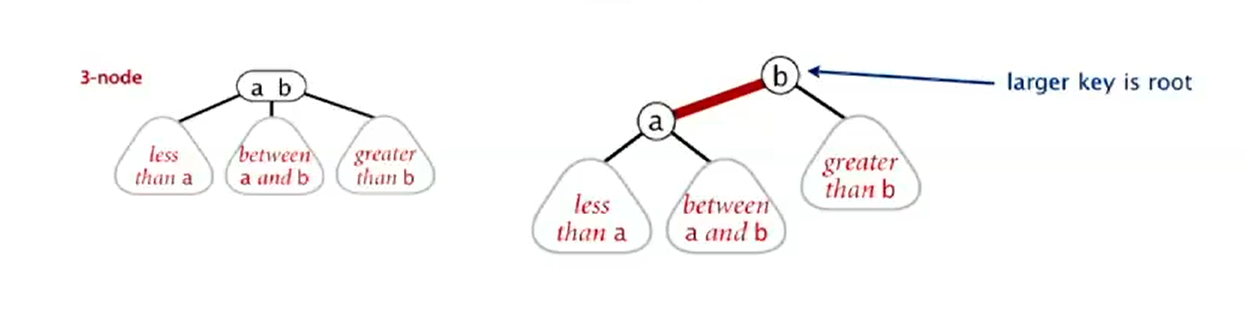
- Black links connect 2-nodes and 3-nodes, red links glue nodes within a 3-node
- Definition: a BST such that
- No node has two read links connected to it
- Perfect black balance: every path from root to null link has the same number of black links
- Red links lean left
- Key property: 1-1 correspondence between 2-3 and LLRB(Left-Leaning
Red-Black Tree)
- Make each red links in LLRB horizontal and replace melt the associated 2-nodes into 3-nodes, the result is a 2-3 tree
- Search implementation: search is the same as for elementary
BST(ignore color)
1
2
3
4
5
6
7
8
9
10
11
12
13
14public Val get(Key key) {
Node x = root;
while (x != null) {
int cmp = key.compareTo(x.key);
if (cmp < 0) {
x = x.left;
} else if(cmp > 0) {
x = x.right;
} else if (cmp == 0) {
return x.val;
}
}
return null;
} - RBT representation
- Since each node is pointed to by precisely one link from its parent,
we can encode color of links in nodes
1
2
3
4
5
6
7
8
9
10
11
12
13
14
15
16
17
18
19
20
21
22
23
24private static final boolean RED = true;
private static final boolean BLACK = false;
private class Node {
private Key key;
private Value val;
private Node left, right;
private boolean color;
private int size;
public Node(Key key, Value val, boolean color, int size) {
this.key = key;
this.val = val;
this.color = color;
this.size = size;
}
}
private boolean isRed(Node x) {
if (x == null) {
return false;
}
return x.color == RED;
}
- Since each node is pointed to by precisely one link from its parent,
we can encode color of links in nodes
- Left rotation: orient a temporarily right-leaning red link to lean
left
- Idea: oldRoot => newRoot.left, oldRoot.right => newRoot
1
2
3
4
5
6
7
8
9
10private Node rotateLeft(Node x) {
Node temp = x.right;
x.right = temp.left;
temp.left = x;
temp.color = x.color;
x.color = RED;
temp.size = x.size;
x.size = size(x.left) + size(x.right) + 1;
return x;
} - Invariants: maintains symmetric order and perfect black balance
- Idea: oldRoot => newRoot.left, oldRoot.right => newRoot
- Right rotation: orient a left-leaning read link to temporarily lean
right
- Idea: oldRoot => newRoot.right, oldRoot.left => newRoot
1
2
3
4
5
6
7
8
9
10private Node rotateLeft(Node x) {
Node temp = x.left;
x.left = temp.right;
temp.right = x;
temp.color = x.color;
x.color = RED;
temp.size = x.size;
x.size = size(x.left) + size(x.right) + 1;
return x;
} - Invariants: maintains symmetric order and perfect black balance
- Idea: oldRoot => newRoot.right, oldRoot.left => newRoot
- Color flip: recolor to split a temporary 4-node
- Idea: middleNode.color: black => red, leftNode.color: red =>
black, rightNode.color: red => black
1
2
3
4
5
6
7
8private void flipColors(Node x) {
assert !isRed(x);
assert isRed(x.left);
assert isRed(x.right);
x.color = RED;
x.left.color = BLACK;
x.right.color = BLACK;
} - Invariants: maintains symmetric order and perfect black balance
- Idea: middleNode.color: black => red, leftNode.color: red =>
black, rightNode.color: red => black
- Insertion in a LLRB tree:
- Basic strategy: maintain 1-1 correspondence with 2-3 trees by applying elementary red-black BST operations
- Every time you insert a new node, it creates a red link with its parent
- Case 1: insert into a 2-node at the bottom
- Prerequisite: insert into a tree with exactly 1 node
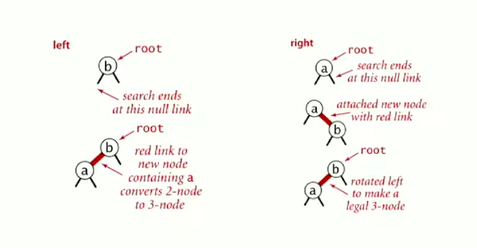
- Steps of insertion:
- Do standard BST insert, color new link red
- If new red link is a right link, do left rotation
- Prerequisite: insert into a tree with exactly 1 node
- Case 2: insert into a 3-node at the bottom
- Prerequisite: insert into a tree with exactly 2 nodes
- Steps of insertion:
- Do standard BST insertion, color new link red
- Rotate to balance the 4-node if needed
- Flip colors to pass red link up one level
- Rotate to make lean left if needed
- Repeat case 1 or 2 up the tree if needed
- Prerequisite: insert into a tree with exactly 2 nodes
- Java implementation
- Handle all cases:
- Right child red, left child black: left rotation
- Left child, left-left grandchild red: right rotation
- Both children red: flip colors
- Java code
1
2
3
4
5
6
7
8
9
10
11
12
13
14
15
16
17
18
19
20
21
22
23
24
25private Node put(Node node, Key key, Value val) {
if (node == null) {
return new Node(key, val, RED);
}
int cmp = key.compareTo(node.key);
if (cmp < 0) {
node.left = put(node.left, key, val);
} else if (cmp > 0) {
node.right = put(node.right, key, val);
} else if (cmp == 0) {
node.val = val;
}
if (isRed(node.right) && !isRed(node.left)) {
node = rotateLeft(node);
}
if (isRed(node.left) && isRed(node.left.left)) {
node = rotateRight(node);
}
if (isRed(node.left) && isRed(node.right)) {
flipColors(node);
}
return node;
}
- Handle all cases:
- Preposition: height or LLRB trees is \(\leq 2logN\) in the worst case
- Performance analysis:
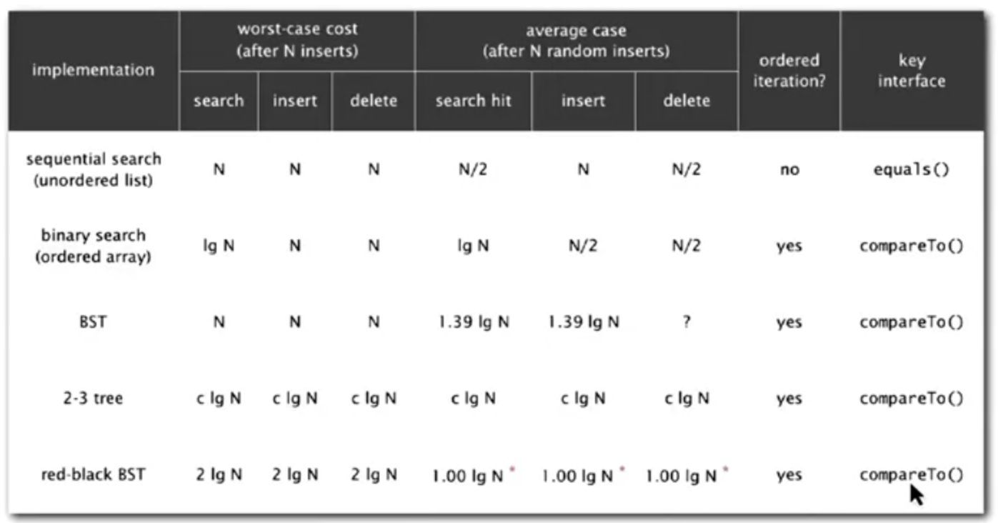
- B-Trees
- Definition: generalize 2-3 trees by allowing up to \(M - 1\) key-link pairs per node
- At least 2 key-link pairs at root
- At least \(M / 2\) key-link pairs in other nodes
- External nodes contain client keys
- Internal nodes contain copies of keys to guide search
- Searching in a B-tree
- Start at root
- Find interval for search key and take corresponding link
- Search terminates in external node
- Insertion in a B-tree
- Search for new key
- Insert at bottom
- Split nodes with M key-link pairs on the way up the tree
- Balance in B-tree
- Preposition: a search or an insertion in a B-tree of order \(M\) with \(N\) keys requires between \(log_{2} {M - 1}\) and \(log_{M / 2} {N}\) probs
- In practice, number of probs is at most 4(M = 1024, N = 62 billion, \(log_{M/2} {N} \leq 4\))
- Optimization: always keep root page in memory
- Balanced trees in the wild
- Red-black trees are widely used as system symbol tables
- Java:
java.util.TreeMap,java.util.TreeSet - C++ STL: map, multimap, multiset
- Linux kernel: completely fair schedule, linux/rbtree.h
- Emacs: conservative stack scanning
- Java:
- B-tree variants: B+ tree, B* tree, B# tree
- B-trees and variants are widely used for file systems and databases
- Windows: NTFS
- Mac: HFS, HFS+
- Linux: ReiserFS, XFS, Ext3FS, JFS
- Databases: ORACLE, DB2, INGRES, SQL, PostgreSQL
- Red-black trees are widely used as system symbol tables
- Definition: generalize 2-3 trees by allowing up to \(M - 1\) key-link pairs per node
- 2-3 Search Trees
- Geometric Applications of BSTs
- 1d Range Search
Extension of ordered symbol table
- Insert key-value pair
- Search for key \(k\)
- Delete key \(k\)
- Range search: find all keys between \(K_1\) and \(k_2\)
- Range count: number of keys between \(k_1\) and \(k_2\)
Application: database queries
Geometric interpretation
- Keys are point on a line
- Find/count points in a given 1d interval
Implementation:
data structure insert range count range search unordered array \(1\) \(N\) \(N\) ordered array \(N\) \(logN\) \(R + logN\) goal \(logN\) \(logN\) \(R + logN\) N = number of keys, R = number of keys that match
1d range search: BST implementation
- Find all keys between
loandhi- Recursively find all keys in left subtree if any could fall in range
- Check key in current node
- Recursively find all keys in right subtree if any could fall in range
- Preposition: running time proportional to \(R + log N\)
- Find all keys between
- Linear Segment Insertion
- Orthogonal line segment insertion search: given \(N\) horizontal and vertical line segments,
find all intersections. Non-degeneracy assumption: all x- and y-
coordinates are distinct
- Quadratic algorithm: check all pairs of line segments for intersection
- Sweep-line algorithm: sweep vertical line from left to right
- x-coordinate define events
- horizontal-segment(left endpoint): insert y-coordinate into BST
- horizontal-segment(right endpoint): remove y-coordinate from BST
- vertical-segment: range search for interval of y-endpoints
- Preposition: the sweep-line algorithm takes time proportional to \(N log N + R\) to find all \(R\) intersections among \(N\) orthogonal line segments
- Orthogonal line segment insertion search: given \(N\) horizontal and vertical line segments,
find all intersections. Non-degeneracy assumption: all x- and y-
coordinates are distinct
- Kd-Trees
- 2d orthogonal range search
- Extension of ordered symbol-table to 2d keys
- Insert a 2d key
- Delete a 2d key
- Search for a 2d key
- Range search: find all keys that lie in a 2d range
- Range count: number of keys that lie in a 2d range
- Geometric interpretation
- Keys are point in the plane
- Find/count points in a given h-v rectangle
- Applications: networking, circuit design, databases
- 2d orthogonal range search: grid implementation
- Divide space into M-by-M grid of squares
- Create list of points contained in each square
- Use 2d array to directly index relevant square
- Insert:
add(x,y)to list for corresponding square - Range search: examine only squares that intersect 2d range query
- Grid implementation is a fast and simple solution for evenly-distributed points, but it does not perform well for when clustering appears
- Extension of ordered symbol-table to 2d keys
- Space-partitioning trees
- Use a tree to represent a recursive subdivision of 2d space
- Grid: divide space uniformly into squares
- 2d tree: recursively divide space into two half-planes
- Quadtree: recursively divide space into four quadrants
- BSP tree: recursively divide space into two regions
- Applications: Ray tracing, 2d range search, nearest neighbor search, collision detections, adaptive mesh generation
- 2d tree
- Data structure: BST, but alternate using x- and y-coordinates as key
- Search gives rectangle containing point
- Insert further subdivides the plane
- Construction
- First level vertical node and then horizontal nodes and then vertical nodes,...
- On the left of previous node => left subtree, on the right of previous node => right subtree
- Range search in a 2d tree: find all points in a query axis-aligned
rectangle
- Check if point in node lies in given rectangle
- Recursively search left/bottom if any could fall in rectangle
- Recursively search right/top if any could fall in rectangle
- Range search performance in a 2d tree
- Typical case: \(R + log N\)
- Worst case: \(R + \sqrt{N}\)
- Nearest neighbor search in a 2d tree: find closest point to the
query point
- Algorithm
- Check distance from point in node to the query point
- Recursively search left/bottom if it could contain a closer point
- Recursively search right/top if it could contain a closer point
- Organize method so that it starts from root
- Algorithm
- Data structure: BST, but alternate using x- and y-coordinates as key
- Flocking boids [Craig Reynolds, 1986]
- Boids, three simple rules lead to complex emergent flocking behavior
- Collision avoidance: point away from k nearest boids
- Flock centering: point towards the center of mass of k nearest boids
- Velocity matching: update velocity to the average of k nearest boids
- Kd tree: recursively partition k-dimensional space into 2
half-spaces
- Implementation: BST, but cycle through dimensions ala 2d trees
- Boids, three simple rules lead to complex emergent flocking behavior
- 2d orthogonal range search
- Interval Search Trees
- 1d interval search: data structure to hold set of overlapping
intervals
- Insert an interval
(lo, hi) - Search for an interval
(lo, hi) - Delete an interval
(lo, hi) - Interval intersection query: given an interval
(lo, hi), find all intervals in data structure that intersects(lo, hi)
- Insert an interval
- 1d interval search API
1
2
3
4
5
6
7public class IntervalST<Key extends Comparable<Key>, Value> {
IntervalST(); // create interval search tree
void put(Key lo, Key hi, Value val); // put interval-value pair into ST
Value get(Key lo, Key hi); // value paired with given interval
void delete(Key lo, Key hi); // delete the given interval
Iterable<Value> intersects(Key lo, Key hi); // all intervals that intersect the given interval
}- Construction
- BST each nodes contains an interval
(lo, hi), use left endpoint as BST key - Store max endpoint in subtree rooted at node
- BST each nodes contains an interval
- Insert an interval
(lo, hi)- Insert into BST, using
loas the key - Update max in each node on search path
- Insert into BST, using
- Find interval that intersects query interval
(lo, hi)- If interval in node intersects query interval, return it
- Else if left subtree is null, go right
- Else is max endpoint in left subtree is less than
lo, go right - Else go left
- Construction
- Interval search tree performance analysis
operation brute interval search tree best in memory insert interval \(1\) \(log N\) \(log N\) find interval \(N\) \(log N\) \(log N\) delete interval \(N\) \(log N\) \(log N\) find any one interval
that intersects(lo, hi)\(N\) \(log N\) \(log N\) find all intervals
that intersects(lo, hi)\(N\) \(R log N\) \(R + log N\) - 1d interval search: data structure to hold set of overlapping
intervals
- Rectangle Intersection
- Orthogonal rectangle intersection search: find all intersections among a set of \(N\) orthogonal rectangles, assume all x- and y-coordinates are distinct
- Use sweep-line algorithm to reduce the problem to 1d interval search
- Proposition: sweep-line algorithm takes time proportional to \(N log N + R log N\) to find \(R\) intersections among a set of \(N\) rectangles
- 1d Range Search

Week 6
- Hash Tables
- Hash Tables
- Hashing: save items in a key-indexed table
- Hash function: method for computing array index from key
- Issues:
- Computing the hash function
- Equality test: method for checking whether two keys are equal
- Collision resolution: algorithm and data structure to handle two keys that hash to the same array index
- Computing the hash function
- Idealistic goal: scramble the keys uniformly to produce a table
index
- Efficiently computable
- Each table index equally likely for each key
- Java
hashCode()function:- Requirement: if
x.equals(y), thenx.hashCode() == y.hashCode() - Highly desirable: if
!x.equals(y), thenx.hashCode() != y.hashCode() - Default implementation: memory address of x
- Customized implementations: Integer, Double, String, File, URL, Date, ...
- String: \(hash = s[0] * 31^{L - 1} + ... + s[L - 1] * 31 ^{0}\)
- User-defined types: users are on their own, a sample hash: \(hash = initialHash + \sum\limits_i {field_i.hashCode()}\)
- Requirement: if
- Modular hashing
- Hash Code: an int between \(- 2^{31}\) and \(2^{31} - 1\)
- Hash function: an int between \(0\)
and \(M - 1\)
1
2
3
4
5
6
7
8
9
10
11
12
13// Wrong, may be negative
private int hash(Key key) {
return key.hashCode() % M;
}
// Wrong, Math.abs() cannot convert - 2 ^31 to 2^31, because Integer.MAX_VALUE is 2 ^31 - 1
private int hash(Key key) {
return Math.abs(key.hashCode()) % M;
}
// Right choice, use 0x7fffffff to remove sign
private int hash(Key key) {
return (key.hashCode() & 0x7fffffff) % M;
}
- Uniform hashing function: each key is equally likely to hash to an
integer between \(0\) and \(M - 1\)
- Bins and balls: throw balls uniformly at random into M bins
- Birthday problem: expect two balls in the same bin after \(\sim \; \sqrt{\pi M / 2}\) tosses
- Coupon collector: expect every bin has \(\geq 1\) ball after \(\sim \; M ln M\) tosses
- Load balancing: After M tosses, expect most loaded bin has \(\Theta(logM / log log M)\) balls
- Bins and balls: throw balls uniformly at random into M bins
- Idealistic goal: scramble the keys uniformly to produce a table
index
- Hashing: save items in a key-indexed table
- Separate Chaining
- Collisions: two distinct keys hashing to same index
- Birthday problem: cannot avoid collisions unless you have a ridiculous amount of memory
- Coupon collector + load balancing: collisions will be evenly distributed
- Separate chaining symbol table: use an array of \(M < N\) linked lists [H. P. Luhn, IBM
1953]
- Hash: map key to integer i between \(0\) and \(M - 1\)
- Insert: put at front of \(i^{th}\) chain if not already here
- Search: need to search only \(i^{th}\) chain
- Proposition: under uniform hashing assumption, prob that the number of keys in a list is within a constant factor of \(N/M\) is extremely close to 1
- ST implementation: summary
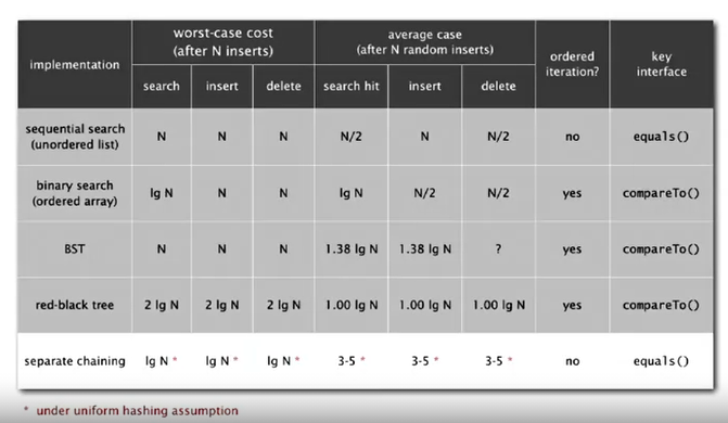
- Collisions: two distinct keys hashing to same index
- Linear Probing
- Collision resolution: open addressing
[Amdahl-Boehme-Rocherster-Samuel, IBM 1953]
- When a new key collides, find next empty slot, and put it there. Put
at table index
iif free, if not tryi + 1,i + 2, etc. - The size M must be greater than number of key-value pairs N, in practice, \(M \geq N * 2\)
- When a new key collides, find next empty slot, and put it there. Put
at table index
- Clustering
- A cluster is a contiguous block of items
- New keys likely to hash into middle of big clusters
- Proposition: under uniform hashing assumption, the average # of probes in a linear probing hash table of size \(M\) that contains \(N = \alpha M\) keys is: \(\sim \frac{1}{2}(1 + \frac{1}{1-\alpha})\) for search hit, and \(\sim \frac{1}{2}(1 + \frac{1}{(1- \alpha)^{2}})\) for search miss or insert. And the typical choice is that \(\alpha = M / N \approx \frac{1}{2}\)
- ST implementation: summary
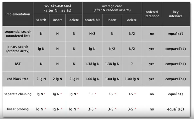
- Collision resolution: open addressing
[Amdahl-Boehme-Rocherster-Samuel, IBM 1953]
- Hash Table Context
- Java 1.1 use skip hashCode in String type, it's unsafe to do so
- Algorithm complexity attacks
- Uniform hashing assumption is important: aircraft control, nuclear reactor, pacemaker
- Denial-of-service attacks
- Diversion: one-way hash functions
- Hard to find a key that will hash to a desired value
- Applications: digital fingerprint, message digest, storing passwords
- Hashing variations:
- Two-probe hashing
- Double hashing
- Cuckoo hashing
- BST v.s. Hash tables
- Hash tables
- Simpler to code
- No effective alternative for unordered keys
- Faster for simple keys
- Better system support in Java for strings
- BST
- Stronger performance guarantee
- Support for ordered ST operations
- Easier to implement
compareTo()correctly thanequals()andhashCode()
- Hash tables
- Hash Tables
- Symbol Table Applications
- Sets: a collection of distinct keys
- API
1
2
3
4
5
6
7
8
9
10
11
12
13
14
15public class SET<Key extends Comparable<Key>> {
// create empty set
SET();
// add the key to the set
void add(Key key);
//is the key in the set?
boolean contains(Key key);
// remove the key from the set
void remove(Key key);
// return the number of keys in the set
int size();
// iterator through keys in the set
Iterator<Key> iterator();
}
- API
- Dictionary Clients
- Build a client to map key to its associated value
- Indexing Clients
- Given a list of files specified, create an index so that you can efficiently find all files containing a given query string
- Sparse Vectors
- For matrix vector multiplication, you can use \(O(N^{2})\) for loop.
- Sparse vector: use symbol table representation(key = index, value = entry) rather than an array can be efficient(array representation space is proportional to N, ST representation is proportional to # of non-zeroes)
- Sparse matrix: each row is a sparse vector rather than an array, space is then proportional to number of non-zeroes plus N rather than \(N^{2}\)
- Sets: a collection of distinct keys